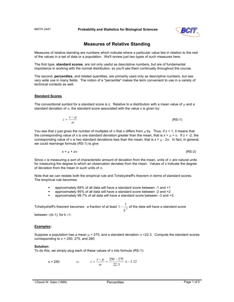
MATH 2441
Probability and Statistics for Biological Sciences
Measures of Relative Standing
Measures of relative standing are numbers which indicate where a particular value lies in relation to the rest
of the values in a set of data or a population. We'll review just two types of such measures here.
The first type, standard scores, are not only useful as descriptive numbers, but are of fundamental
importance in working with the normal distribution, so you'll see them continually throughout the course.
The second, percentiles, and related quantities, are primarily used only as descriptive numbers, but see
very wide use in many fields. The notion of a "percentile" makes the term convenient to use in a variety of
technical contexts as well.
Standard Scores
The conventional symbol for a standard score is z. Relative to a distribution with a mean value of  and a
standard deviation of , the standard score associated with the value x is given by:
z
x
(RS-1)

You see that z just gives the number of multiples of  that x differs from  by. Thus, if z = 1, it means that
the corresponding value of x is one standard deviation greater than the mean; that is x =  + . If z = -2, the
corresponding value of x is two standard deviations less than the mean; that is x =  - 2. In fact, in general,
we could rearrange formula (RS-1) to give
x =  + z
(RS-2)
Since  is measuring a sort of characteristic amount of deviation from the mean, units of  are natural units
for measuring the degree to which an observation deviates from the mean. Values of z indicate the degree
of deviation from the mean in such units of .
Note that we can restate both the empirical rule and Tchebysheff's theorem in terms of standard scores.
The empirical rule becomes:



approximately 68% of all data will have a standard score between -1 and +1
approximately 95% of all data will have a standard score between -2 and +2
approximately 99.7% of all data will have a standard score between -3 and +3.
Tchebysheff's theorem becomes: a fraction of at least 1 
1
k2
of the data will have a standard score
between (k-1), for k 1.
Examples:
Suppose a population has a mean  = 275, and a standard deviation  =22.3. Compute the standard scores
corresponding to x = 250, 275, and 280.
Solution:
To do this, we simply plug each of these values of x into formula (RS-1):
x = 250
David W. Sabo (1999)

z
x


250  275
 1.12
22 .3
Percentiles
Page 1 of 5
x = 275

x = 280

x
275  275
0

22 .3
x   280  275
z

 0.224

22 .3
z

Notice that the mean value always gives a standard score of zero.

Question: What is the standard score of a value which is 1.5 standard deviations above the mean?
Answer: We could answer this question by substitution into the formula (RS-1). After all, a value x which is
1.5 standard deviations above the mean would have the value
x =  + 1.5
Thus,
z
x


(   1.5 )  


  1.5   1.5

 1.5


However, you may have been able to answer this question with z = 1.5 without doing any calculations by just
recalling the definition of the standard score as the number of standard deviations the data value differs from
the mean.

Percentiles, Deciles, Quartiles
The notion of a percentile is quite simple: the pth -percentile for a set of data or a population is the value
which is greater than or equal to p% of the data or population, but is less than or equal to (100 - p)% of the
data or population. So, it is a value which divides the data or population into two parts: the lower p% of the
values and the upper (100-p)% of the values.
Then deciles are just percentiles that are multiples of 10. So the first decile is the 10 th percentile, and is a
value which divides a population or set of data into the lower 10% of the values and the upper 90%. The
second decile is the 20th percentile, dividing the data into a lower 20% and an upper 80% and so on.
Quartiles are the only other specially named percentiles, being those for which p is a multiple of 25. Thus:



the first quartile or lower quartile or Q1 is the 25th percentile, the value separating the
elements of a population or set of data into the lower 25% and the upper 75%.
the second quartile is the 50th percentile, which we've already encountered as the median.
the third quartile or upper quartile or Q3 is the 75th percentile.
Associated with the notion of quartiles is the interquartile range or IQR:
IQR = Q3 - Q1
(RS-3)
the difference between the upper and lower quartiles. This is a single number that gives the width of the
interval of values into which the middle 50% of the data or population fall. The IQR plays a similar role with
respect to the median that the standard deviation does with respect to the mean (though the IQR is more
like 2 in this respect).
Quite often people report results (such as test scores) as percentiles rather than the original raw data values
when they want to indicate how an observation rates in relation to other observations, but don't want to
attribute any concrete meaning to the actual original data values. Thus aptitude test scores are often stated
as percentiles. From one version of the test to another, actual grades may vary up or down in general
because the questions change. Thus, the actual test grades are not seen to be as meaningful as how a
particular person scores in relation to everyone else who wrote that test. A person who scores in the 90th
percentile on one test is seen to have displayed comparable aptitude to a person who scored in the 90 th
percentile on a different version of the test, even though their actual grades might have been different in part
Page 2 of 5
Percentiles
David W. Sabo (1999)
because different questions posed differing levels of difficulty. Percentiles are used when the focus is on
how one element of a set of data or a population rates relative to the others: near the top, in the middle,
near the bottom.
These defining ideas are quite simple and intuitive. The trouble starts when we ask how these various
percentile values are to be calculated for finite sets of data or finite populations.
You might think that if we had exactly 100 distinct values in our set of data, there would be no problem. We
would just sort them in order from smallest to biggest. Then, the first (smallest) value would be the first
percentile, because it is equal to or greater than 1% of the values in the set. The next (second smallest)
would be the second percentile, and so on up. Unfortunately, even in this special case, things aren't quite
that simple. After all, any number between the smallest and the second smallest data value satisfies the
definition of being the first percentile. Further, if we use this approach all the way up, we find that when we
get to the 50th percentile, the result doesn't agree with our previous definition of the median, which is defined
to be equivalent to the 50th percentile. The point of this example is that the application of the simple
conceptual definition of percentiles is a bit ambiguous for data sets or populations of finite size.
Rather than get bogged down in a discussion of too many possible variations, we will explain one common
approach to calculating sample percentiles which we will use in the course, and just mention one variation
that you need to watch out for. To calculate the p th percentile of a set of n data values, proceed as follows:
1.
sort the data values from smallest to largest. The smallest will be labeled
x1 , and on up, so that the largest is labeled xn.
2.
compute the number: m 
3.
p
(n  1) . Do not round your result to a
100
whole number. This will be called the index number of the pth percentile
for the n-member data set.
If m is a whole number, then the pth percentile is xm. If m is not a whole
number, do linear interpolation (illustrated in the example below).
This procedure gives a 50th percentile which is identical to our previous definition of the
median. Again, this is just one of several approaches, but it is a common approach.
Also, as the size of the data set increases, the results of the various procedures
become more and more similar.
Example SalmonCa0:
We'll use the data set SalmonCa0 to illustrate the procedure to calculate the 10 th
percentile (Q1), the 50th percentile, and Q3. The n = 40 values are shown to the right
already sorted into increasing order, with index numbers in the first column.
So, the index number for the 10th percentile is:
m
10
40  1  4.1
100
This is not an integer. The index value, m = 4.1, means that we need to calculate a
value that lies 0.1 of the way between x4 and x5. Because both x4 and x5 have the
value 52, the result will be 52. Formally though, to calculate the required number, we
would write:
10th percentile = x4 + 0.1(x5 - x4)
= 52 + 0.1(52 - 52) = 52
So, the 10th percentile for this set of data is the value 52.
Q1 is the same as the 25th percentile. Thus, the index number for Q1 is
David W. Sabo (1999)
Percentiles
1.
2.
3.
4.
5.
6.
7.
8.
9.
10.
11.
12.
13.
14.
15.
16.
17.
18.
19.
20.
21.
22.
23.
24.
25.
26.
27.
28.
29.
30.
31.
32.
33.
34.
35.
36.
37.
38.
39.
40.
29
43
47
52
52
53
54
54
56
56
59
61
61
63
63
67
68
68
68
69
72
72
72
73
75
76
78
83
88
90
91
94
96
101
101
103
107
107
120
129
Page 3 of 5
m
25
40  1  10 .25
100
Thus, Q1 is the value 0.25 of the way between x10 and x11:
Q1 = x10 + 0.25(x11 - x10)
= 56 + 0.25(59 - 56) = 56.75
The median is the 50th percentile, and so corresponds to the index number
m
50
40  1  20 .5
100
x is the value halfway between x20 and x21. The linear interpolation approach gives exactly the same
Thus, ~
result in this case as calculating the mean of x20 and x21:
~
x  x 20  0.5x 21  x 20 
= 69 + 0.5(72 - 69) = 70.5.
In the same way, you will find that the index number for Q3, the upper quartile, is 30.75, and so doing the
linear interpolation, we get Q3 = 90.75.
By the way, since we now have values for both Q1 and Q3, we can calculate the interquartile range for this
data:
IQR = Q3 - Q1 = 90.75 - 56.75 = 34.

Most of the alternative ways of computing percentiles for finite-sized sets of data handle the situation where
the index number is not an integer in different ways. The one place you will encounter quite a different
approach overall is when you use the QUARTILE() function available in Microsoft Excel. That function
calculates the index number using the formula
m  1
p
n  1
100
and does linear interpolation if m is not a whole number. This formula still gives agreement between the 50th
percentile and the median. The other unique feature it has is that the smallest data value becomes the 0 th
percentile, and the largest value becomes the 100th percentile.
(The procedure we gave earlier doesn't make sense of either the 0th percentile or the 100th percentile. If you
like, it indicates that the 0th percentile is smaller than the smallest value present, and the 100 th percentile is
larger than the largest value present. This has a certain logic to it when you are using sample percentiles to
estimate population percentiles because it is unlikely that a small random sample of a much larger
population will contain both the smallest and the largest elements of that population.)
Excel's approach amounts to focussing on the gaps between the data values more so than on the data
values themselves. For relatively small sets of data, the Excel version of percentiles can be quite different
from those using other approaches.
As a matter of interest, for the SalmonCa0 data, Excel gives Q1 = 58.25 and Q3 = 90.25 .
Some references define quantities called hinges, which are usually very similar in value to quartiles. The
general intent seems to be that the lower hinge represents the midpoint between the median and the
smallest data value or that it is the midpoint of the lower half of the data (and so should be very similar to the
lower quartile, Q1, in value). Similarly, the upper hinge represents the midpoint between the median and
the largest data value or the midpoint of the upper half of the data (and so should be very similar to the
upper quartile, Q3, in value). There are differences in the way in which various authors propose the
calculation of hinge values, but most procedures give roughly the same values, which are also usually quite
Page 4 of 5
Percentiles
David W. Sabo (1999)
similar to the values of the corresponding quartiles. For this reason, in this course we will continue to use
quartiles where some other authors may make use of hinges.
(Many basic statistics textbooks make no mention of hinges at all. If you wish to follow up on the notion a
little bit, you will find some discussion in Anderson, Sweeney and Williams, Introduction to Statistics, 3rd
edition, 1993: page 69, and Mendenhall & Beaver, Introduction to Probability and Statistics, 9th edition,
1994: pages 91-94. The concept may have originated with the statistician John Tukey, and you can find his
view in his book, Exploratory Data Analysis, 1977, pages 32-33, including a brief rationalization of the term
"hinge.")
David W. Sabo (1999)
Percentiles
Page 5 of 5