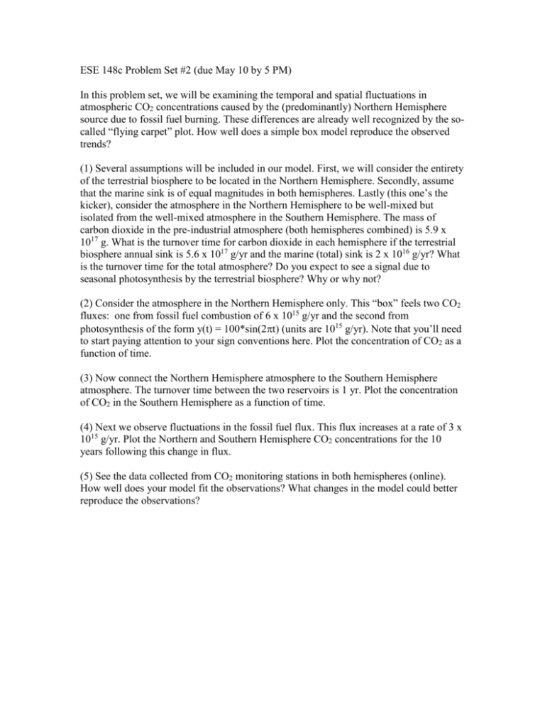
ESE 148c Problem Set #2 (due May 10 by 5 PM)
In this problem set, we will be examining the temporal and spatial fluctuations in
atmospheric CO2 concentrations caused by the (predominantly) Northern Hemisphere
source due to fossil fuel burning. These differences are already well recognized by the socalled “flying carpet” plot. How well does a simple box model reproduce the observed
trends?
(1) Several assumptions will be included in our model. First, we will consider the entirety
of the terrestrial biosphere to be located in the Northern Hemisphere. Secondly, assume
that the marine sink is of equal magnitudes in both hemispheres. Lastly (this one’s the
kicker), consider the atmosphere in the Northern Hemisphere to be well-mixed but
isolated from the well-mixed atmosphere in the Southern Hemisphere. The mass of
carbon dioxide in the pre-industrial atmosphere (both hemispheres combined) is 5.9 x
1017 g. What is the turnover time for carbon dioxide in each hemisphere if the terrestrial
biosphere annual sink is 5.6 x 1017 g/yr and the marine (total) sink is 2 x 1016 g/yr? What
is the turnover time for the total atmosphere? Do you expect to see a signal due to
seasonal photosynthesis by the terrestrial biosphere? Why or why not?
(2) Consider the atmosphere in the Northern Hemisphere only. This “box” feels two CO2
fluxes: one from fossil fuel combustion of 6 x 1015 g/yr and the second from
photosynthesis of the form y(t) = 100*sin(2t) (units are 1015 g/yr). Note that you’ll need
to start paying attention to your sign conventions here. Plot the concentration of CO2 as a
function of time.
(3) Now connect the Northern Hemisphere atmosphere to the Southern Hemisphere
atmosphere. The turnover time between the two reservoirs is 1 yr. Plot the concentration
of CO2 in the Southern Hemisphere as a function of time.
(4) Next we observe fluctuations in the fossil fuel flux. This flux increases at a rate of 3 x
1015 g/yr. Plot the Northern and Southern Hemisphere CO2 concentrations for the 10
years following this change in flux.
(5) See the data collected from CO2 monitoring stations in both hemispheres (online).
How well does your model fit the observations? What changes in the model could better
reproduce the observations?