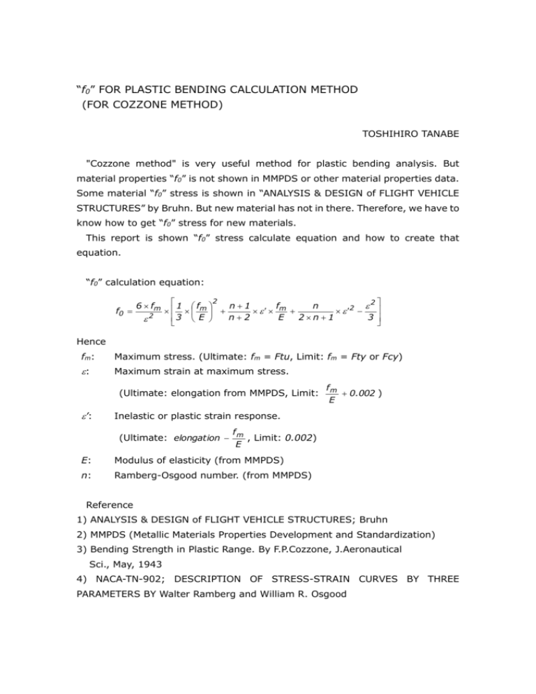
“f0” FOR PLASTIC BENDING CALCULATION METHOD
(FOR COZZONE METHOD)
TOSHIHIRO TANABE
"Cozzone method" is very useful method for plastic bending analysis. But
material properties “f0” is not shown in MMPDS or other material properties data.
Some material “f0” stress is shown in “ANALYSIS & DESIGN of FLIGHT VEHICLE
STRUCTURES” by Bruhn. But new material has not in there. Therefore, we have to
know how to get “f0” stress for new materials.
This report is shown “f0” stress calculate equation and how to create that
equation.
“f0” calculation equation:
f0 
6  fm
2
 1  f 2 n  1
f
n
2 

  m 
   m 
  2 
n2
E
2n1
3
3  E 


Hence
fm:
Maximum stress. (Ultimate: fm = Ftu, Limit: fm = Fty or Fcy)
:
Maximum strain at maximum stress.
(Ultimate: elongation from MMPDS, Limit:
’:
fm
 0.002 )
E
Inelastic or plastic strain response.
(Ultimate: elongation 
fm
, Limit: 0.002)
E
E:
Modulus of elasticity (from MMPDS)
n:
Ramberg-Osgood number. (from MMPDS)
Reference
1) ANALYSIS & DESIGN of FLIGHT VEHICLE STRUCTURES; Bruhn
2) MMPDS (Metallic Materials Properties Development and Standardization)
3) Bending Strength in Plastic Range. By F.P.Cozzone, J.Aeronautical
Sci., May, 1943
4) NACA-TN-902; DESCRIPTION OF STRESS-STRAIN CURVES BY THREE
PARAMETERS BY Walter Ramberg and William R. Osgood
How to create “f0” equation
The Cozzone method is replaces the true bending variation curve by a
trapezoidal stress variation. The stress “f0” is fictions stress which is assumed
exist at the neutral axis or at zero strain. The value of “f0” is determined by
making the requirement that the internal moment of the true stress variation
must equal the moment of the assumed trapezoidal stress variation.


FMAX = fm
f0
N.A.
f0

FMAX = fm
fm

fm
N.A.

2
0
fm
f0

Equation “f0” strain
 
 f 
f

    
E
 fm 
f0   

2
n
 fm  f0  
EQ. (1)

2


2
   f  d
0
3

(Rectangle area moment) (Triangle area moment)

f0   2
2
 fm  f0  
 f  d
0
2
3

EQ. (2)
From equation (1)
d
1 n     f n  1
 
df
E
fmn
 1 n     f n  1 
df
d   
n
E

fm


Therefore
f
n     f n 
f d   
df
E

fmn


EQ. (3)
From equation (1) & (3)
n
n

 f   f
 f  
f
    n     
 df
f  d       
E
 fm    E
 fm  

EQ. (4)
2

3
From equation (3)
u
0
n
n


 

 
 f      f    f  n      f  df
 f   E
f  
0 E
 m  
 m 

2n 
fm  f  2

n  1     f n  1
2  f  



 n 
df
  

0  E 
E  fm
 fm  

f  d 

fm

EQ. (5)
fm
1 f3
n1
f n  2 
n
f 2n  1 
 

  

  2 

2
n2
E  fmn 2  n  1
fm2n 0
 3 E

1 fm3 n  1
f 2
n


   m 
  2  fm
2
3 E
n2
E
2n1
From equations (2) & (5)
2
f0   2
2
1
n1
f
n
f 
 fm  f0  
  fm   m  
    fm  m 
  2  fm
2
3
3
E
n

2
E
2
n

1


 1  f 2 n  1

f0
f
f
n
  2  m   2  fm     m  
   m 
  2 
6
3
n2
E
2n1
3  E 



Therefore
f0 
6  fm
2
 1  f 2 n  1
f
n
2 

  m 
   m 
  2 
n2
E
2n1
3
3  E 


Equation check result
Comparison of Reference(1) “f0” values and equation results.
Ref.(1)
Fig No
Material
Thickness
Ftu
in
ksi
Fty
E ×103
e
f0u
f0y
ksi
%
ksi
ksi
Calc. value
f0u
f0y
ksi
ksi
C3.9
2024-T3C SHT
0.01~0.062
59
39
9.5
15
50
18
50
16
C3.11
2024-T4C PLT
0.25~0.50
62
40
10.0
15
55
20
52
17
C3.13
2024-T3 SHT
~0.25
64
42
10.5
15
53
23
54
18
C3.15
7075-T6C SHT
~0.39
70
60
10.0
5
64
24
62
22
C3.17
7075-T6 EXT
~0.25
75
65
10.4
7
70
29
68
24
C3.16
7075-T6 SHT
~0.039
76
65
10.3
7
70
24
69
24
Calculated values are almost same as Reference 1) “f0” values.