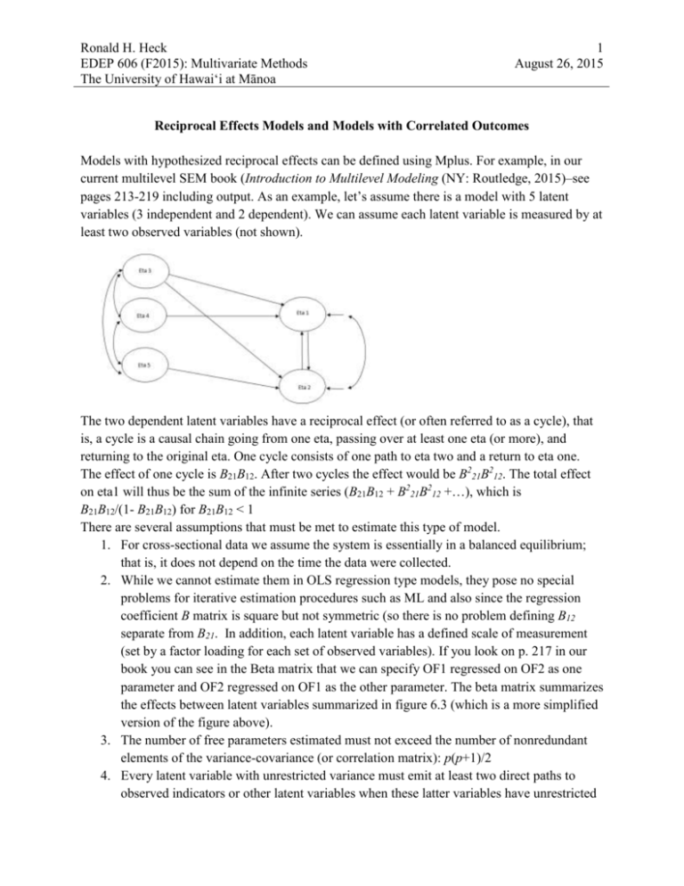
Ronald H. Heck
EDEP 606 (F2015): Multivariate Methods
The University of Hawai‘i at Mānoa
1
August 26, 2015
Reciprocal Effects Models and Models with Correlated Outcomes
Models with hypothesized reciprocal effects can be defined using Mplus. For example, in our
current multilevel SEM book (Introduction to Multilevel Modeling (NY: Routledge, 2015)–see
pages 213-219 including output. As an example, let’s assume there is a model with 5 latent
variables (3 independent and 2 dependent). We can assume each latent variable is measured by at
least two observed variables (not shown).
The two dependent latent variables have a reciprocal effect (or often referred to as a cycle), that
is, a cycle is a causal chain going from one eta, passing over at least one eta (or more), and
returning to the original eta. One cycle consists of one path to eta two and a return to eta one.
The effect of one cycle is B21B12. After two cycles the effect would be B221B212. The total effect
on eta1 will thus be the sum of the infinite series (B21B12 + B221B212 +…), which is
B21B12/(1- B21B12) for B21B12 < 1
There are several assumptions that must be met to estimate this type of model.
1. For cross-sectional data we assume the system is essentially in a balanced equilibrium;
that is, it does not depend on the time the data were collected.
2. While we cannot estimate them in OLS regression type models, they pose no special
problems for iterative estimation procedures such as ML and also since the regression
coefficient B matrix is square but not symmetric (so there is no problem defining B12
separate from B21. In addition, each latent variable has a defined scale of measurement
(set by a factor loading for each set of observed variables). If you look on p. 217 in our
book you can see in the Beta matrix that we can specify OF1 regressed on OF2 as one
parameter and OF2 regressed on OF1 as the other parameter. The beta matrix summarizes
the effects between latent variables summarized in figure 6.3 (which is a more simplified
version of the figure above).
3. The number of free parameters estimated must not exceed the number of nonredundant
elements of the variance-covariance (or correlation matrix): p(p+1)/2
4. Every latent variable with unrestricted variance must emit at least two direct paths to
observed indicators or other latent variables when these latter variables have unrestricted
Ronald H. Heck
EDEP 606 (F2015): Multivariate Methods
The University of Hawai‘i at Mānoa
2
August 26, 2015
Reciprocal Effects Models and Models with CO
5. error variances. Typically we correlate the error variances between the variables in the
reciprocal relationship. This comes from the idea that if eta1 and eta2 mutually cause
each other they are mutually affected by omitted variables (i.e., the residuals). Note they
must also not have exactly the same set of predictors. So you will see in the diagram, we
propose some independent latent variables do not affect eta1 and some do not affect eta2.
More specifically, each latent variable in the feedback loop has some latent variables that
affect it outside the feedback loop and some that don’t. More specifically, the number of
variables excluded for each variable in the feedback look has to be greater than the total
number of endogenous variables in the model minus 1. In this case, there are two
endogenous variables so there must be at least one independent variable excluded from
each. So, you can see the model in the figure works because each dependent latent
variable has only 2 independent latent variables predicted it.
Unfortunately, you cannot run this model in SPSS using multiple regression, since the modeling
of reciprocal effects calls for maximum likelihood estimation and the ability to define both
dependent variables at once. Below is an example of a reciprocal effects model you can run in
Mplus with observed variables. It is saturated (or just identified), as there are two intercepts for
the y variables that are also estimated. If I don’t estimate them, the model will have two degrees
of freedom and the parameters change just slightly. Reciprocal effects models typically require
that the model is in equilibrium (i.e., it is stable). Also, it is important that you have one predictor
that does not affect each salary outcome in order for the model to estimate (i.e., since there are
two endogenous variables). I estimated this using the data set we are using in Chapter 2
regarding path models.
You can contrast the reciprocal effects formulation above with a model where you just assume
the two salary variables are correlated. If you run the model in SPSS, you can actually get the
results to match the Mplus results by saving the standardized residuals for each regression
Ronald H. Heck
EDEP 606 (F2015): Multivariate Methods
The University of Hawai‘i at Mānoa
3
August 26, 2015
Reciprocal Effects Models and Models with CO
equation (i.e., the model predicting beginning salary and the model predicting current salary).
Then you just correlate the residuals and you get the same 0.787 that Mplus estimates. The data
set is the SPSS file “employee” data.