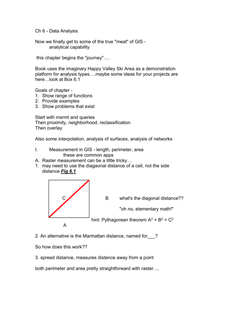
Ch 6 - Data Analysis
Now we finally get to some of the true "meat" of GIS analytical capability
this chapter begins the "journey"….
Book uses the imaginary Happy Valley Ski Area as a demonstration
platform for analysis types….maybe some ideas for your projects are
here…look at Box 6.1
Goals of chapter 1. Show range of functions
2. Provide examples
3. Show problems that exist
Start with msrmt and queries
Then proximity, neighborhood, reclassification
Then overlay
Also some interpolation, analysis of surfaces, analysis of networks
I.
Measurement in GIS - length, perimeter, area
these are common apps
A. Raster measurement can be a little tricky…
1. may need to use the diagaonal distance of a cell, not the side
distance Fig 6.1
C
B
what's the diagonal distance??
"oh no, elementary math!"
hint: Pythagorean theorem A2 + B2 = C2
A
2. An alternative is the Manhattan distance, named for___?
So how does this work??
3. spread distance, measures distance away from a point
both perimeter and area pretty straightforward with raster….
Ch 6 - p.2
Vector GIS uses Pythag theorem to get distance Fig 6.2.
Also, the line and perimeter data can be entered as attribute data (you
see this in AV all the time).
B. Queries (we've done some of these with the "Query Builder" in AV…
Book says performing queries is an "essential part" of many GIS
projects
two diff types of queries defined here:
1. spatial
2. aspatial (attribute-driven) - example could be, what is the street
name?
Boolean operators are used to build more complicated queries involving
AND, OR, NOT, and either/or.
C. reclassification of features
pretty easy to do with raster - example of reclassifying a complex image
with one part of it being forest (originally 10, new class = 1), and
reclassfying everything else as = 0. So all that is left is forest = 1, and
eveything else = 0. So you can see how this is a bit like a query asking
for "forest".
II.
Buffering and neighborhood functions
An entity can influence its neighbors, or the neighbors can influence the
entity. This happens several ways:
Buffering - create a "zone of interest" around an entity Fig 6.4
Do for pts lines or polygons
Filtering - recalculate value of a raster cell based upon value of its
neighbors.
A. Buffering example - find names of all hotels within 200m of a main
road…how do this?
"More than one method of achieving an answer."
One way - make a buffer zone 200 m, then use a point in polygon
overlay.
Ch 6 p.3
Second way - measure distance from the main road to each hotel, ID
those less than 200 m away.
We'll see how to do a buffer in AV. Much easier to do buffer in vector
than in raster, where proximity map is made. Fig 6.5
B. Filtering example - used often for remote sensing imagery. Filter is
passed across each raster cell, and the original value is
recalculated. This operation tends to smooth "noisy data".
III.
Map Overlay - way to integrate data
"ability to integrate data from two sources using map overlay is perhaps
the key GIS analysis function"
take two different thematic layers, overlay them, and create a new layer
modern techniques date back to McHarg (1969), though geologists
have been overlaying maps and making calculations for well over 100
years….
Map overlay has many applications…sometimes just placing vector
data on top of raster data.
But usually overlay is more analytical, like combining several diff factors
to search for the best position for a ski slope, for example.
Overlay in vector system is complex and time-consuming - in raster, it is
simple and efficient.
A. Vector overlay
Several diff types (Fig 6.7) including point in polygon, line in
polygon, polygon on polygon
Note that with vector, your output will always be more complex:
more lines, polygons, etc.
Several examples shown in Fig 6.7  point in polygon allows land use attributes to be joined with rain
gauge attributes (visual version of a table join…)
Ch 6 p.4
 line in polygon - as with points, but there are new line segments
ID'd in order to accommodate new attributes brought in due to
overlay process itself - Fig 6.7
 polygon on polygon - 3 diff outputs result from overlay oprns 1. output layer has all polygons from both input maps - this is
from the Boolean operator OR (known as a UNION)
2. this output shows all lands within the resort area - this is a
Boolean operator known as ERASE (known as a cookiecutter) - here, the operation erases everything that is NOT
resort
3. this output meets both criteria, so it is an AND operation
(known as an INTERSECTION)
pay attention here - it is easy to get confused as to the nature of these
operations - the naming is not intuitive
B. Raster Overlay
Raster overlay quite diff than vector - Fig 6.10 - numbers are
assigned to describe cell attributes
Then math oprns are performed upon cells within each layer - add,
subtract, etc.
Note how the point in poly, line in poly, poly on poly oprns all results
in diff cell values ( fig 6.10)
Look at fig 6.10a as example of point in polygon….add the rain
gauge station cells to the resort cells and get a range of values what do these mean? Think of the operation being
performed….here, an addition….that is, gauge AND resort (an
intersection)
Fig 6.10b - same thing as a.
6.10c - a variety of oprns shown
good point at end of this section about scales of msrmt and
nonsensical output…must be careful to keep track of the NOIR
scales of msrmt - don't mix apples with oranges
Ch 6 - p.5
IV. Spatial interpolation
Process involves estimating values at points where no data currently
exists - this of course is the whole process of mapping
Whole idea behind mapping is to predict values, geology,
contaminant patterns, whatever, in an area based upon your map.
Height or elevation contours are typical of how we use maps to
predict values…..contour map represents how a horizontal line can
be traced around a 3D object: use some surveyed-in USGS
benchmark elevations and a bunch of stereo air photos to make
topo maps:
X 400'
X 300 '
X 400 '
X 500'
x 300'
X 400'
x 300'
This shows a hill slope dropping from 500 feet above sea level to
300 feet above sea level
Important to remember that any map is an interpretation product it's your best guess of reality, but no guarantee that it IS reality…
Book touches on a few methods of interpretation - including
Thiessen polygons, triangulated irregular networks TINs, spatial
moving average. Plate 12
Thiessen and TIN both require building polygons or triangles to
model the 3D surface you're mapping, while spatial moving average
is bit more like how your brain would be looking at this data in 3D,
and drawing a more contour-like surface.
Ch 6 p.6
V.Analysis of Surfaces
Slope, aspect, and visibility are 3 of the more common GIS
automated packages to look at slopes.
What is slope? Just like you learned in math….rise over run. In the field,
often measured in degrees, like with a Brunton compass….
0o = horizontal surface
90o = vertical surface
Aspect = direction toward which a slope faces (N,S,E,W, etc) fig 6-11
Why visibility analysis? Used a lot for locating radio transmitters, TV
towers, cell phone towers….can predict where the dead zones are to be
found. Fig 6-12
This is how a viewshed map is built
VI. Network Analysis Very valuable with certain occupations, like fire fighters, police, EMS
responders - also, truckers, shipping companies, anyone who's trying to
find the most economical way to get from pt A to pt B.
What's the definition? " A set of interconnected lines….through which
resources can flow"
Several "classic" network problems:
 ID the shortest path
 "travelling salesperson"
 allocation modeling
 route tracing
A. shortest path - remember that shortest in distance may NOT be
shortest in time….especially in New York and New Jersey!!!
The GIS analyst is looking for the route with the "least impedance"
B. travelling salesperson
must plan out the route efficiently to see all clients in one day….
C. location / allocation
"matching supply with demand"
D. route tracing
Good for unidirectional (one way) flow. Streams, sewer sytems,
one way streets….directionality and connectivity are key.