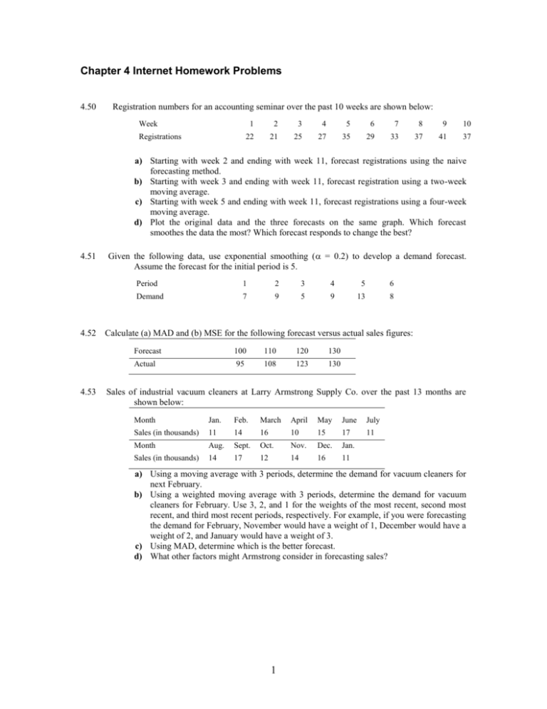
Chapter 4 Internet Homework Problems
4.50
Registration numbers for an accounting seminar over the past 10 weeks are shown below:
Week
Registrations
1
2
3
4
5
6
7
8
9
10
22
21
25
27
35
29
33
37
41
37
a) Starting with week 2 and ending with week 11, forecast registrations using the naive
forecasting method.
b) Starting with week 3 and ending with week 11, forecast registration using a two-week
moving average.
c) Starting with week 5 and ending with week 11, forecast registrations using a four-week
moving average.
d) Plot the original data and the three forecasts on the same graph. Which forecast
smoothes the data the most? Which forecast responds to change the best?
4.51
Given the following data, use exponential smoothing ( = 0.2) to develop a demand forecast.
Assume the forecast for the initial period is 5.
Period
1
2
3
4
5
6
Demand
7
9
5
9
13
8
4.52 Calculate (a) MAD and (b) MSE for the following forecast versus actual sales figures:
4.53
Forecast
100
110
120
130
Actual
95
108
123
130
Sales of industrial vacuum cleaners at Larry Armstrong Supply Co. over the past 13 months are
shown below:
Month
Jan.
Feb.
March
April
May
June
July
Sales (in thousands)
11
14
16
10
15
17
11
Month
Aug.
Sept.
Oct.
Nov.
Dec.
Jan.
Sales (in thousands)
14
17
12
14
16
11
a) Using a moving average with 3 periods, determine the demand for vacuum cleaners for
next February.
b) Using a weighted moving average with 3 periods, determine the demand for vacuum
cleaners for February. Use 3, 2, and 1 for the weights of the most recent, second most
recent, and third most recent periods, respectively. For example, if you were forecasting
the demand for February, November would have a weight of 1, December would have a
weight of 2, and January would have a weight of 3.
c) Using MAD, determine which is the better forecast.
d) What other factors might Armstrong consider in forecasting sales?
1
4.54 Passenger miles flown on Northeast Airlines, a commuter firm serving the Boston hub, are shown for
the past 12 weeks:
Week
1
2
3
4
5
6
Actual Passenger Miles
17
21
19
23
18
16
Week
7
8
9
10
11
12
Actual Passenger Miles
20
18
22
20
15
22
(in thousands)
(in thousands)
a) Assuming an initial forecast for week 1 of 17,000 miles, use exponential smoothing to
compute miles for weeks 2 through 12. Use α = .2.
b) What is the MAD for this model?
c) Compute the RSFE and tracking signals. Are they within acceptable limits?
4.55
4.56
Given the following data, use least squares regression to derive a trend equation. What is your
estimate of the demand in period 7? In period 12?
Period
1
2
3
4
5
6
Demand
7
9
5
11
10
13
Joe Barrow, owner of Barrow’s Department Store, has used time-series extrapolation to forecast
retail sales for the next 4 quarters. The sales estimates are $120,000, $140,000, $160,000,
and $180,000 for the respective quarters. Seasonal indices for the 4 quarters have been
found to be 1.25, .90, .75, and 1.10, respectively. Compute a seasonalized or adjusted sales
forecast.
4.57 The director of the Riley County, Kansas, library system would like to forecast evening patron usage
for next week. Below are the data for the past 4 weeks:
Week 1
Week 2
Week 3
Week 4
Mon
Tue
Wed
Thu
Fri
Sat
210
215
220
225
178
180
176
178
250
250
260
260
215
213
220
225
160
165
175
176
180
185
190
190
a) Calculate a seasonal index for each day of the week.
b) If the trend equation for this problem is y= 201.74 + .18x, what is the forecast for each day of week 5?
Round your forecast to the nearest whole number.
2
4.58 A careful analysis of the cost of operating an automobile was conducted by a firm. The following
model was developed:
Y = 4,000 + 0.20X
where Y is the annual cost and X is the miles driven.
a) If the car is driven 15,000 miles this year, what is the forecasted cost of operating this
automobile?
b) If the car is driven 25,000 miles this year, what is the forecasted cost of operating this
automobile?
4.59 The following multiple-regression model was developed to predict job performance as measured by a
company job performance evaluation index based on a preemployment test score and
college grade point average (GPA):
Y = 35 + 20X1 + 50X2
where
Y = job performance evaluation index
X1 = preemployment test score
X2 = college GPA
a) Forecast the job performance index for an applicant who had a 3.0 GPA and scored 80
on the preemployment score.
b) Forecast the job performance index for an applicant who had a 2.5 GPA and scored 70
on the preemployment score.
4.60
A study to determine the correlation between bank deposits and consumer price indices in
Birmingham, Alabama, revealed the following (which was based on n = 5 years of data):
x = 15
x2 = 55
xy = 70
y = 20
y2 = 130
a) What is the equation of the least square regression line?
b) Find the coefficient of correlation. What does it imply to you?
c) What is the standard error of the estimate?
3
4.61 The accountant at Rick Wing Coal Distributors, Inc., in San Francisco notes that the demand for coal
seems to be tied to an index of weather severity developed by the U.S. Weather Bureau.
When weather was extremely cold in the U.S. over the past 5 years (and the index was thus
high), coal sales were high. The accountant proposes that one good forecast of next year’s
coal demand could be made by developing a regression equation and then consulting the
Farmer’s Almanac to see how severe next year’s winter would be. For the data in the
following table, derive a least squares regression and compute the coefficient of correlation
of the data. Also compute the standard error of the estimate.
Coal Sales, y
4
1
4
6
5
2
1
4
5
3
(in millions of tons)
Weather Index, x
4.62 Given the following data, use least squares regression to develop a relation between the number of
rainy summer days and the number of games lost by the Boca Raton Cardinal baseball team.
Year
Rainy Days
Games Lost
1994
1995
1996
1997
1998
1999
2000
2001
2002
2003
15
25
25
20
10
10
10
15
30
20
20
15
20
20
15
10
10
5
25
20
4