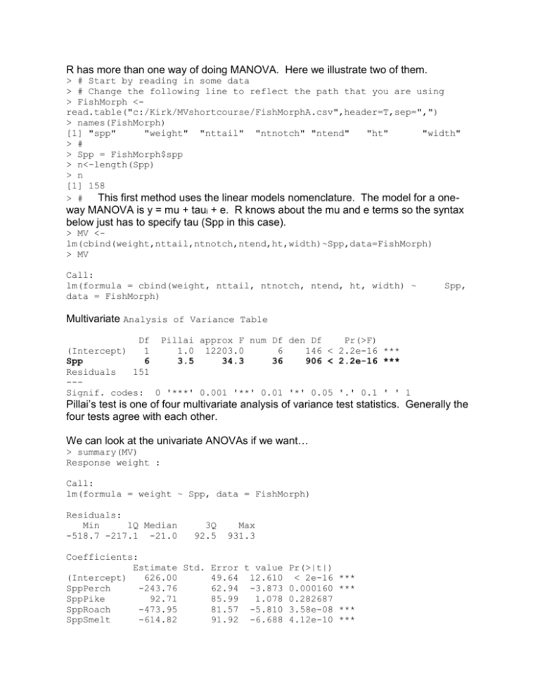
R has more than one way of doing MANOVA. Here we illustrate two of them.
> # Start by reading in some data
> # Change the following line to reflect the path that you are using
> FishMorph <read.table("c:/Kirk/MVshortcourse/FishMorphA.csv",header=T,sep=",")
> names(FishMorph)
[1] "spp"
"weight" "nttail" "ntnotch" "ntend"
"ht"
"width"
> #
> Spp = FishMorph$spp
> n<-length(Spp)
> n
[1] 158
> #
This first method uses the linear models nomenclature. The model for a one-
way MANOVA is y = mu + taui + e. R knows about the mu and e terms so the syntax
below just has to specify tau (Spp in this case).
> MV <lm(cbind(weight,nttail,ntnotch,ntend,ht,width)~Spp,data=FishMorph)
> MV
Call:
lm(formula = cbind(weight, nttail, ntnotch, ntend, ht, width) ~
data = FishMorph)
Spp,
Multivariate Analysis of Variance Table
Df Pillai approx F num Df den Df
Pr(>F)
(Intercept)
1
1.0 12203.0
6
146 < 2.2e-16 ***
Spp
6
3.5
34.3
36
906 < 2.2e-16 ***
Residuals
151
--Signif. codes: 0 '***' 0.001 '**' 0.01 '*' 0.05 '.' 0.1 ' ' 1
Pillai’s test is one of four multivariate analysis of variance test statistics. Generally the
four tests agree with each other.
We can look at the univariate ANOVAs if we want…
> summary(MV)
Response weight :
Call:
lm(formula = weight ~ Spp, data = FishMorph)
Residuals:
Min
1Q Median
-518.7 -217.1 -21.0
3Q
92.5
Max
931.3
Coefficients:
Estimate Std. Error t value Pr(>|t|)
(Intercept)
626.00
49.64 12.610 < 2e-16 ***
SppPerch
-243.76
62.94 -3.873 0.000160 ***
SppPike
92.71
85.99
1.078 0.282687
SppRoach
-473.95
81.57 -5.810 3.58e-08 ***
SppSmelt
-614.82
91.92 -6.688 4.12e-10 ***
SppWhBream
SppWhitefsh
-471.18
-95.00
100.41
128.18
-4.693 6.00e-06 ***
-0.741 0.459759
There are seven species, but only 6 tauhats—the seventh is gotten by subtraction
noting that all of the tauhats sum to zero.
--Signif. codes:
0 '***' 0.001 '**' 0.01 '*' 0.05 '.' 0.1 ' ' 1
Residual standard error: 289.5 on 151 degrees of freedom
Multiple R-Squared: 0.375,
Adjusted R-squared: 0.3501
F-statistic: 15.1 on 6 and 151 DF, p-value: 1.694e-13
Etc…
Now let’s look at the second approach…
The discriminant analysis below requires the “MASS” library.
>
> library(MASS)
>
This version of MANOVA uses the “analysis of variance” nomenclature.
> MV2 <manova(cbind(weight,nttail,ntnotch,ntend,ht,width)~Spp,data=FishMorph)
> MV2
Call:
manova(cbind(weight, nttail, ntnotch, ntend, ht, width) ~ Spp,
data = FishMorph)
Terms: The following summarizes the univariate sums of squares
Spp Residuals
weight
7591083 12652952
nttail
9493
6285
ntnotch
11056
7076
ntend
13352
7909
ht
10418
388
width
633
184
Deg. of Freedom
6
151
Residual standard error: 289.4726 6.451375 6.845388 7.237116 1.603757
1.104316
Estimated effects may be unbalanced
> summary(MV2)
Df Pillai approx F num Df den Df
Pr(>F)
Spp
6 3.460
34.291
36
906 < 2.2e-16 ***
Residuals 151
--Signif. codes: 0 '***' 0.001 '**' 0.01 '*' 0.05 '.' 0.1 ' ' 1
Note that the results for the two analyses are the same.
I fooled MANOVA into printing out the sums of squares and cross-products matrix for
error. Note that the diagonal values are the individual ANOVA error sums of squares.
> E <- (n-1)*cov(MV2$residuals)
> E
weight
nttail
ntnotch
ntend
ht
width
weight 12652952.27 266468.6005 283427.5298 299861.9836 28303.1991 18269.9951
nttail
266468.60
6284.6554
6664.9178
7041.3401
595.0382
377.5523
ntnotch
283427.53
6664.9178
7075.7609
7475.5016
638.5748
405.3956
ntend
299861.98
7041.3401
7475.5016
7908.7532
675.4037
431.7763
ht
28303.20
595.0382
638.5748
675.4037
388.3774
148.0163
width
18270.00
377.5523
405.3956
431.7763
148.0163
184.1465
I also fooled R into printing out the sums of squares and cross-products matrix for
species (treatments). Note that the diagonal values are the univariate ANOVA sums of
squares for species or treatments.
> H <- (n-1)*cov(MV2$fitted.values)
> H
weight
nttail
ntnotch
ntend
ht
width
weight 7591083.294 251469.8081 273576.9453 306640.7184 62192.7004 -1147.0814
nttail
251469.808
9493.4530 10240.9515 11130.3078 -137.9448 -267.8547
ntnotch 273576.945 10240.9515 11055.9815 12044.8959
125.3972 -239.9840
ntend
306640.718 11130.3078 12044.8959 13352.1863 1330.5677 -279.7009
ht
62192.700
-137.9448
125.3972
1330.5677 10417.9113 1206.9191
width
-1147.081
-267.8547
-239.9840
-279.7009 1206.9191
632.8826
The four multivariate test statistics, including Pillai’s test, depend on the eigenvalues of
HE-1.
> roots<-eigen(H%*%solve(E))$values
> roots
[1] 5.478328e+01 9.295249e+00 3.736631e+00 1.287332e+00 2.877527e-01 3.015442e-04
R’s MANOVA does not have a convenient function for getting the t-1 = 6 canonical
variates associated with the analysis. However, the linear discriminant functions are
proportional to the canonical variates.
> #
> dis<-lda(FishMorph[,-1],Spp,prior = c(1,1,1,1,1,1,1)/7)
> dis
Call:
lda(FishMorph[, -1], Spp, prior = c(1, 1, 1, 1, 1, 1, 1)/7)
Coefficients of linear discriminants:
CanVar1LD1 CanVar2LD2 Etc. LD3
LD4
LD5
LD6
weight
0.0007552994 0.005407768 -0.006394442 -0.002494222 -0.005972577 -0.003256034
nttail
0.1850420685 1.444298977 -1.537010678 0.587209254 3.054392531 -3.062164748
ntnotch 1.6591660467 0.845843015 3.225632501 1.407882218 -3.414268010 3.032594136
ntend
-1.7226673515 -2.377492352 -1.425475748 -1.724661065 0.666842986 -0.108563161
ht
-0.6866328962 0.190938581 0.070635366 0.298739353 -0.006109224 -0.027016533
width
0.3554321014 0.242471837 0.534579037 -0.829018685 0.260004147 -0.142753909
The number of interpretable canonical variables is determined by looking at
the relative magnitude of the eigenvalues above. It appears that there is
one very strong canonical variate and perhaps a second one is interpretable.
We would like to calculate the correlations between CanVar1 and CanVar2 with
each of the original variables, but I haven’t figured out yet how to do that
.