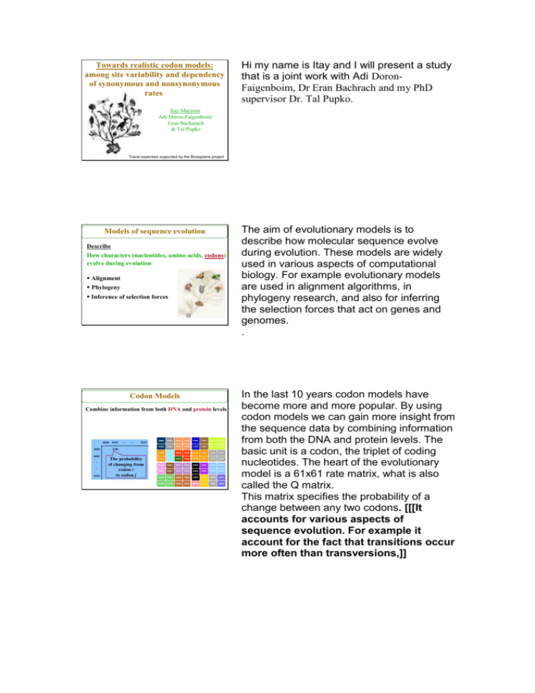
Towards realistic codon models:
among site variability and dependency
of synonymous and nonsynonymous
rates
Hi my name is Itay and I will present a study
that is a joint work with Adi DoronFaigenboim, Dr Eran Bachrach and my PhD
supervisor Dr. Tal Pupko.
Itay Mayrose
Adi Doron-Faigenboim
Eran Bacharach
& Tal Pupko
Travel expenses supported by the Biosapiens project
Models of sequence evolution
Describe
How characters (nucleotides, amino acids, codons)
evolve during evolution
 Alignment
 Phylogeny
 Inference of selection forces
Codon Models
Combine information from both DNA and protein levels
AAA
AAA
AAC
…
…
CCC
AAC
…
…
CCC
AAC
ACA
ACC
CAA
CAC
CCA
CCC
AAG
AAU
ACG
ACU
CAG
CAU
CCG
CCU
AGA
AAA
AGC
AUA
AUC
CGA
CGC
CUA
CUC
AGG
AGU
AUG
AUU
CGG
CGU
CUG
CUU
GAA
GAC
GCA
GCC
UAA
UAC
UCA
UCC
GAG
GAU
GCG
GCU
UAG
UAU
UCG
UCU
GGA
GGC
GUA
GUC
UGA
UGC
UUA
UUC
GGG
GGU
GUG
GUU
UGG
UGU
UUG
UUU
0.09
The probability
of changing from
codon i
to codon j
The aim of evolutionary models is to
describe how molecular sequence evolve
during evolution. These models are widely
used in various aspects of computational
biology. For example evolutionary models
are used in alignment algorithms, in
phylogeny research, and also for inferring
the selection forces that act on genes and
genomes.
.
In the last 10 years codon models have
become more and more popular. By using
codon models we can gain more insight from
the sequence data by combining information
from both the DNA and protein levels. The
basic unit is a codon, the triplet of coding
nucleotides. The heart of the evolutionary
model is a 61x61 rate matrix, what is also
called the Q matrix.
This matrix specifies the probability of a
change between any two codons. [[[It
accounts for various aspects of
sequence evolution. For example it
account for the fact that transitions occur
more often than transversions,]]
Codon Models
Combine information from both DNA and protein levels
Synonymous
(silent )
Non-synonymous
(amino-acid altering)
AAA
AAA
AAC
…
…
CCC
AAC
…
…
CCC
AAC
ACA
ACC
CAA
CAC
CCA
CCC
AAG
AAU
ACG
ACU
CAG
CAU
CCG
CCU
AGA
AAA
AGC
AUA
AUC
CGA
CGC
CUA
CUC
AGG
AGU
AUG
AUU
CGG
CGU
CUG
CUU
GAA
GAC
GCA
GCC
UAA
UAC
UCA
UCC
GAG
GAU
GCG
GCU
UAG
UAU
UCG
UCU
GGA
GGC
GUA
GUC
UGA
UGC
UUA
UUC
GGG
GGU
GUG
GUU
UGG
UGU
UUG
UUU
0.09
The probability
of changing from
codon i
to codon j
Codon Models
Combine information from both DNA and protein levels
Synonymous
(silent )
Non-synonymous
(amino-acid altering)
AAA
 Purifying evolution
 Neutral evolution
 Positive Darwinian
evolution
AAC
ACA
ACC
CAA
CAC
CCA
CCC
AAG
AAU
ACG
ACU
CAG
CAU
CCG
CCU
AGA
AGC
AUA
AUC
CGA
CGC
CUA
CUC
AGG
AGU
AUG
AUU
CGG
CGU
CUG
CUU
GAA
GAC
GCA
GCC
UAA
UAC
UCA
UCC
GAG
GAU
GCG
GCU
UAG
UAU
UCG
UCU
GGA
GGC
GUA
GUC
UGA
UGC
UUA
UUC
GGG
GGU
GUG
GUU
UGG
UGU
UUG
UUU
Detecting selection pressure
S1 AAG ACT GCC GGG CGT ATT
S2 AAA ACA GCA GGA CGA ATC
S1 K T A G R I
S2 K T A G R I
Synonymous = 6
Non-synonymous = 0
Purifying selection:
Non-synonymous << Synonymous substitutions
Histones
But the most important use of codon
models is that now [[using this matrix]] we
can differentiate between two kinds of
substitution rates: the synonymous, or silent,
substitution rate, are those between two
codons that do not change the amino acid.
Usually these are substitutions at the third
position of the codon. In addition, we get the
non-synonymous rate, substitutions that
cause a change in the coded amino-acid.
By contrasting these two types of rates we
can infer not only if a protein position is
conserved, under purifying selection, or
variable, under no selection, but also and
what is unique to codon models is the
inference of positive adaptive evolution.
So, for example, if one observes that all
substitutions in a gene are silent – here 6
substitutions are synonymous and zero
nonsynonymous, so the encoded protein is
completely conserved. This means that the
protein is under strong purifying selection.
The most known example is the histone
family where there is very strong purifying
selection at the protein level. And indeed all
observed substitutions are silent.
Detecting selection pressure
S1 AAG ACT GCC GGG CGT ATT
S2 AAA ACA GAC GGA CAT ATG
S1 K T A G R I
S2 K T D G H M
Synonymous = 3
Non-synonymous = 3
Neutral selection:
Non-synonymous = Synonymous substitutions
Detecting selection pressure
S1 AAG ACT GCC GGG CGT ATT
S2 AAT ATT GAC GAG CAT ATG
S1 K T A G R I
S2 N I D E H M
Synonymous = 0
Non-synonymous = 6
Positive (Darwinian) selection :
Non-synonymous >> Synonymous substitutions
Host-pathogen arm-race
The Ka/Ks ratio
Synonymous
substitution rate
Non-synonymous
substitution rate
Assume: Ks = neutral rate of evolution
Ka/Ks < 1Purifying selection: 
Ka/Ks = 1Neutral selection: 
Ka/Ks > 1Positive selection: 
In some cases the rates of nonsynonymous
and non-synonymous substitutions are
equal. In this case, we assume that the
synonymous substitution rate corresponds to
the neutral rate of evolution and so the
protein is under neutral evolution or no
selection.
In exceptional cases, almost all observed
nucleotide substitutions change also the
coded amino acids, so the number of nonsynonymous substitutions is significantly
higher than the number of synonymous
substitutions. This is indicative for a situation
where it is beneficial for a protein to change
and may point to a protein that is under
positive selection.
For example, it was found that positive
selection operates in proteins involved in
host-pathogen arm-race. HIV is a classical
example, where certain positions are under
positive selection, which allows the virus to
escape the host immune system.
Formally, the synonymous substitution rate
is termed Ks and the non-synonymous rate
is termed Ka. If we assume that Ks
represents the neutral evolutionary rate then
we compute the Ka/Ks rate ratio and infer
the type of selection. So purifying selection
is inferred when the KaKs rate ratio is
significantly lower than 1. And positive
selection is inferred when this ratio is
significantly higher than 1.
Existing codon models
Assume:
Ka varies over sites
Ks is the same for all sites and reflects the
neutral rate of evolution
•Goldman & Yang (1994)
•Muse & Gaut (1994)
Almost all existing codon evolutionary
models assume that the Ka rate can vary
between sites due to selection at the protein
level. In contrast, these models assume that
there is no selection at the DNA level and so
the synonymous rate is the same for all
sites.
•Nielsen & Yang (1998)
•Wong, Sainudiin & Nielsen (2006)
•Doron-Faigenboim & Pupko (2007)
Existing codon models
Assume:
I will call this model KaV-KsC for variable Ka
and constant Ks.
Ka varies over sites
Ks is the same for all sites and reflects the
neutral rate of evolution
Model name: KaV-KsC
•Goldman & Yang (1994)
•Muse & Gaut (1994)
•Nielsen & Yang (1998)
•Wong, Sainudiin & Nielsen (2006)
•Doron-Faigenboim & Pupko (2007)
Existing codon models
Assume:
Ka varies over sites
Ks is the same for all sites and reflects the
neutral rate of evolution
Ks constant?
•Goldman & Yang (1994)
•Muse & Gaut (1994)
•Nielsen & Yang (1998)
•Wong, Sainudiin & Nielsen (2006)
•Doron-Faigenboim & Pupko (2007)
The question is if this assumption, which
states that the Ks is the same for all
positions, is valid and truly represents the
biological reality.
There are several indications that this is not
the case.
Existing codon models
Assume:
Ka varies over sites
Ks is the same for all sites and reflects the
neutral rate of evolution
For example, the group of Svante Paabo
have estimated that around 40% of
synonymous sites in primates are subject to
purifying selection
Ks constant?
Hellmann et al. (2003):
Approximately 39% of synonymous sites in
primates are subject to purifying selection
Selection against silent substitutions
Human
Mouse
Dog
GAG GCT GCC GGG CGT ATT
GGC ACT GCC GGG CGT ATT
GGG ACT GCC GGG CGT ATT
 RNA stability
 Exonic splicing regulatory sequences
 RNA editing
 Overlapping genes
 Codon bias and GC content
 Translational efficiency
 Protein folding
Reviewed in
Chamary, Parmley, and Hurst
Nature Reviews Genetics (2006)
Evolutionary models for Ks conservation
Pond & Muse: both Ka and Ks can vary
(two independent gamma distributions)
Model name: KaV-KsV
Pond and Muse
Mol Biol Evol (2005)
“Site-to-site variation of synonymous substitution rates”
Conservation of synonymous sites may
result from various kinds of selection
pressure.
For example, in the mRNA, there are some
sites, especially those in the stem regions,
that are important for maintaining the RNA
stability.
There are of course other kinds of selection:
splicing regulatory elements, RNA editing,
overlapping genes, codon bias, translation
efficiency.
And even few months ago it was shown
that a synonymous substitution change
the rate of translation and results in a
protein with a completely different 3D
structure.
A main challenge is how to capture the
selection on synonymous sites within the
evolutionary model. Recently Pond & Muse
have presented an evolutionary model in
which both the Ka and Ks rates can vary
over sites.
Technically they assumed that the Ka and
ks rates are sampled from two
independent rate distributions.
I will call this model KaV-KsV as both Ka
and Ks can vary between sites.
Evolutionary models for Ks conservation
The KaV-KsV model assumes:
Each position evolves independently
But:
• Selection is often regional
• Site-specific Ka and Ks are very erratic
4
3.5
3
2.5
2
1.5
1
0.5
0
50
100
150
200
Evolutionary models for Ks conservation
The KaV-KsV model assumes:
Each position evolves independently
But:
• Selection is often regional
• Site-specific Ka and Ks are very erratic
4
3.5
Ka
True
Ks
3
2.5
Ka/Ks
1.0 1.0
2
1.0
Estimated 1.2 1.5
0.8
1.5
Similar to most evolutionary models, this
model assumes that each site along a
sequence evolves independently.
But selection forces, especially those that
influence synonymous sites, are often
regional. In addition, because the estimated
Ka/Ks values are now a ratio of two inferred
quantities, inference inaccuracies can
quickly lead to very erratic estimates.
For example: let’s say that we are looking at
a neutrally evolving site with both Ka and Ks
equal 1. Random fluctuations in the
sequences can easily shift the inference of
Ka to be 1.2 and the inference of Ks to 0.8.
The inferred ka/ks ratio for this site will be
1.5 which is a signature of positive selection.
1
0.5
0
50
100
150
200
Evolutionary models for Ks conservation
The KaV-KsV model assumes:
Each position evolves independently
But:
• Selection is often regional
• Site-specific Ka and Ks are very erratic
4
Our solution: 3.5
3
Incorporate site-dependencies
2.5
2
1.5
1
0.5
0
50
100
150
200
So how can we solve this erratic behavior?
One option is to use a sliding window
approach to smooth the inferred rates. But a
more statistically robust approach is to
incorporate the biological phenomena that
adjacent positions have similar rates into the
evolutionary model.
Modeling dependencies among sites
Ka at position n depends on the Ka at position n-1
&
Ks at position n depends on the Ks at position n-1
Two HMM chains
Ka
0.1
0.3
0.8
0.7
0.2
Ks
1.3
0.8
1.0
0.7
0.1
TCA
TCC
TAC
GCC
GCG
GCC
ATC
ATC
ATC
Hidden states
CTT
CTA
CTG
Observations
GGG
GGG
GAA
Modeling dependencies among sites
Ka at position n depends on the Ka at position n-1
&
Ks at position n depends on the Ks at position n-1
So in our suggested model the Ka at
position n depends on the Ka at position n-1
& similarly for Ks.
This dependency is incorporated into the
model by assuming two hidden markov
models, or HMMs. One represents the
variation of Ka along the sequence and the
other the variation of ks. So now, if the Ka
rate at the first position is 0.1 then there is a
higher chance that position 2 will have a
similar Ka rate. The technical details of the
model are presented in the paper, so I won’t
cover them here.
We call this model KaD-KsD as both rates
are dependent among adjacent positions.
Model name: KaD-KsD
Two HMM chains
Ka
0.1
0.3
0.8
0.7
0.2
Ks
1.3
0.8
1.0
0.7
0.1
TCA
TCC
TAC
GCC
GCG
GCC
ATC
ATC
ATC
Hidden states
CTT
CTA
CTG
Observations
GGG
GGG
GAA
Comparing the models
Models tested
• KaV-KsC: Variable nonsynonymous
Constant synonymous
• KaV-KsV: Variable nonsynonymous
Variable synonymous
• KaD-KsD: Dependent nonsynonymous
Dependent synonymous
So to summarize, we want to compare
between 3 models: the first which is the
most simple and also the most widely used
ignores the possibility of Ks variation.
The second assumes that both the Ka and
Ks rates can vary. This model ignores the
spatial correlation of rates.
And finally our model, which accounts for
both dependency and variability of the Ka
and Ks rates.
To compare these 3 models we have
analyzed the 9 coding genes of HIV-1.
We chose HIV because it is a well known
example to have sites evolving under
positive selection. Also in viruses, because
of their compact genome we expect to find
more selection at the DNA level.
For each gene of HIV-1 multiple sequence
alignment were downloaded from the Los
Alamos HIV database. For each dataset a
phylogenetic tree was created. And then the
parameters of each model were optimized
until convergence of the likelihood function.
Using the likelihood ratio test we then tested
if the increase in likelihood is statistically
justified when moving from the simple to the
more complex ones.
Comparing the models
For each of the 9 coding genes of HIV-1:
Multiple sequence alignment
Phylogenetic tree
Parameters optimization
Model comparison (LRT)
HIV-1 data
Accounting for Ks
variability is
extremely justified
for all HIV-1 genes
HIV-1 genes exhibit a
strong pattern of rate
dependency
HIV-1
gene
Log-likelihood difference
from KaV-KsC
KaV−KsV
KaD−KsD
env
914
1080
gag
362
nef
339
380
pol
1346
1565
rev
228
248
tat
214
228
vif
239
279
vpr
130
154
vpu
188
197
409
Difference of 5 log-likelihoods is significant (p < 0.01)
This table shows the difference in loglikelihood for each gene compared between
the constant ks model and the two models
that allow for Ks variation. Difference of 5
log-likelihood points between the models is
considered significant.
As you can see the differences in loglikelihoods between the models for all HIV-1
genes is very high, in the order of hundreds.
So it is clear that accounting for Ks variability
is extremely well supported.
In addition, accounting for the dependencies
between adjacent Ka and Ks rates is also
highly justified.
Now, the comparison between log-likelihood
values tells which model is best supported
by each gene but it doesn’t tell us if we can
gain more biological insights when using a
more complex model. So the question is
“does it really matter which model to use?”
Inferring sites under positive selection
KaV-KsC
491
KaV-KsV
295
41
66
310
135
53
5
13
1. The most conservative
2. With the highest overlap
with the other models
KaD-KsD
206
True positive rate
Inferring sites under positive selection
KaV-KsV
KaD-KsD
0.8
0.6
0.4
KaV-KsC
0.2
0
0
0.1
0.2
False positive rate
0.3
One of the main reasons to use codon
models is to detect sites that are under
positive selection pressure.
As can be sees in the Venn diagram, the
inference of positive selection is very
sensitive to the specific model used.
For example, when inferring positive
selection over the entire HIV-1 genome the
standard kaV-ksC model infers almost 500
sites as being positively selected.
However, when taking into account the
variation of Ks that number drops to around
300 and when the spatial correlation is
considered the estimated number is even
more conservative and is only 206 sites.
This is an encouraging property because the
inference of positive selection is often
blamed to have a high number of false
positives.
In addition, the dependency model has the
highest overlap with the 2 other models
which also suggests that this model has less
false positives. Of course, we don’t really
know which sites are true positives or true
negatives. So we also used computer
simulations to check which of the models is
more accurate for inferring positively
selected sites.
I won’t get into the details of the simulations,
but using a ROC curve we can test which
model is more precise. As the curve is closer
to the upper left corner the prediction is
more accurate. It is clear from this graph that
the standard model, which ignores Ks
variability is the least accurate. And that the
KaD-KsD model is the most accurate. This
result was repeated under various simulation
scenarios.
Identifying cis regulatory elements
21 stretches in HIV-1 are under significant
Ks selection
region
Pol
17 matched to
known functional
regions
Function
898-947 DNA flap + cPPT + CTS
Pol 986-1003
Overlap Vif
Vif
173-186
Overlap Vpr
Nef
88-99
3’ PPT
Tat
41-51
Overlap Rev
Env
728-744
Pol
7-31
?
Vif
1-21
Overlap pol
Overlap Tat & Rev
…
The most significantly conserved Ks region
is located around the center of the HIV
genome inside the pol open reading frame.
This region spans about 150 bp or 50
codons.
Conservation of Ks in pol
4
Ks rate
Using our model we can compute the Ka
and Ks for each site. We next used the
estimates of Ks to search for linear stretches
that have a significantly reduced Ks values.
These stretches are good candidates to
have a functional role at the DNA or RNA
levels.
We searched for such conserved Ks
stretches across the whole HIV genome and
found 21 regions. The first few are listed
here. Of these suspected regions we could
correlate 17 to known functional elements,
or to regions with gene overlap.
3
2
1
0
750
800
850
900
950
Position
Conservation of Ks in pol (zoom in)
Ks rate
4
DNA flap
3
CTS
2
1
?
cPPT
0
900
910
920
930
Position
940
950
If we zoom into this region, we can see a cluster
of functional elements.
The most conserved region - on the left - is
called the central polypurine tract (cPPT). This
region serves as a primer for DNA synthesis in
the process of reverse transcription.
On the right, there is a functional element called
the Central Termination Sequence, or the CTS,
which is the site where DNA synthesis stops.
In between these two elements, there is the DNA
flap region, which is a complex DNA structure
that is composed of three DNA strands. This
DNA flap structure was only recently discovered
and it was found to contribute for the import of
the HIV genome to the nucleus. The exact
positions that are critical for the function of the
DNA flap are still unknown. By analyzing the Ks
variation in this graph it seems that some
positions are more conserved than others so
these may be the more important ones.
Finally, beyond the CTS there is another region
with a marked reduction of Ks. However, we
could not find evidence for the importance of this
region in the literature. [[and we predict that is
functionally important as well]]
Conservation of Ks in pol (zoom in)
DNA flap
Ks rate
4
3
CTS
2
cPPT
1
If we continue downstream from this
conserved region we see another area with
very low Ks values.
This area exactly maps to the overlapped
region of pol with vif.
0
900
920
940
960
980
1000
Position
pol-vif overlap
4
Ka
Ks
Rate
3
vif
2
1
vif and pol overlap
but with different
reading frames
When we look at the two genes together we
see that the end of pol and the beginning of
vif both have very low Ks rate.
0
0
20
40
Position
Ka
4
Ks
pol
Rate
3
2
1
These regions
exhibit a
substantial
reduction of Ks
0
950
970
990
Position
pol-vif overlap
Site 12
4
Ka
Ks
Rate
3
vif
2
1
0
0
20
40
Position
Ka
Rate
4
Ks
pol
3
2
1
0
950
970
Position
990
Site 12 of vif has
very high Ks.
Why?
What is a bit surprising is site #12 in vif,
which is part of the overlapped region but
has a quite high ks rate.
pol-vif overlap
pol
Site 999 in pol
is under strong
positive selection
(Ka/Ks = 11.4)
Ka
Ks
3
Rate
vif
Site 12 of vif has
very high Ks.
Why?
Site 12
4
2
1
0
0
20
40
Position
Ka
Rate
4
Ks
Site 999
3
2
1
0
950
970
990
Position
Selection at overlapping regions
21 stretches in HIV-1 are under significant
Ks selection
region
Pol
Function
898-947 DNA flap + cPPT + CTS
Pol 986-1003
Overlap Vif
Vif
173-186
Overlap Vpr
Nef
88-99
3’ PPT
Tat
41-51
Overlap Rev
Env
728-744
Pol
7-31
?
Vif
1-21
Overlap Pol
When we looked for a possible explanation
we observed that the corresponding position
in pol, site 999, has a high non-synonymous
rate, with a KaKs ratio of 11.4, which is
indicative of positive selection. So in this
case we suggest that the positive selection
at site 999 is responsible for the marked
increase of ks in site 12 of vif.
So here again, by obtaining both the Ka
and Ks rates we can gain interesting
biological insights that we could have
ignored if we used the standard model
which assume constant Ks.
Overall, when we look at the conserved
stretches that are under significant Ks
conservation we can explain a large fraction
of them due to such overlapped regions.
Overlap Tat & Rev
…
Selection at overlapping regions
Overlapped regions exhibit significant Ks
conservation
1.5
overlap
non-overlap
1
0.5
0
Ks
p-value < 10-6
Ka
Comparing the Ks values of the overlapped
regions with those at the non-overlapped
regions we see that on average overlapped
position have a lower synonymous rate. This
is quite expected because of the constraints
imposed by the overlapped gene.
Selection at overlapping regions
Overlapped regions exhibit significant Ks
conservation
1.5
overlap
non-overlap
1
But:
significant
Ka
variability
0.5
0
Ks
What was quite surprising is that the Ka at
overlapped regions tends to have higher
non-synonymous rate. This may mean that
at the protein level the overlapped regions
are less important.
Ka
p-value < 10-6
Next…
Analyze specific Ks stretches in details
Study Ks selection in other viruses
Examine the extent of Ks selection
across different lineages
What is the meaning of the Ka/Ks>1 criterion?
How should positive selection be defined?
To conclude, we believe that the integration
of Ks variability into evolutionary models can
be very helpful in studying various types of
selection pressures.
Our most immediate plan is to
experimentally analyze the most conserved
regions that we have found in HIV and don’t
have an assigned function yet.
We also plan to apply this model to other
viruses that are less well annotated.
In addition we would like to study the extent
and source of selection on synonymous
sites in different phylogenetic groups. For
example, we want to analyze the amount of
Ks conservation in mammals compared to
viruses and bacteria. And in each phyla to
analyze the sources of this selection: so in
mammals splicing regulation or RNA editing
may be more important, and in bacteria
maybe the efficiency of translation is the
most important factor.
Finally, there is a theoretical difficulty that I
didn’t get into in this talk. This difficulty is
related to the definition of positive selection.
When positive selection is inferred using the
Ka/Ks ratio we assume that Ks is free from
selection and represents the neutral
evolutionary rate. But as I just showed, in
many cases this is not true. This leads to the
question of how should we define and detect
positive selection. In mammals it is possible
to use introns to estimate the neutral rate of
evolution. But if we go back to viruses where
the inference of positive selection is very
important – this criterion remains undefined.
Next…
Analyze specific Ks stretches in details
Thank you
Study Ks selection in other viruses
Examine the extent of Ks selection
across different lineages
What is the meaning of the Ka/Ks>1 criterion?
How should positive selection be defined?
So I will leave this question open and I
would like to thank you very much for
listening