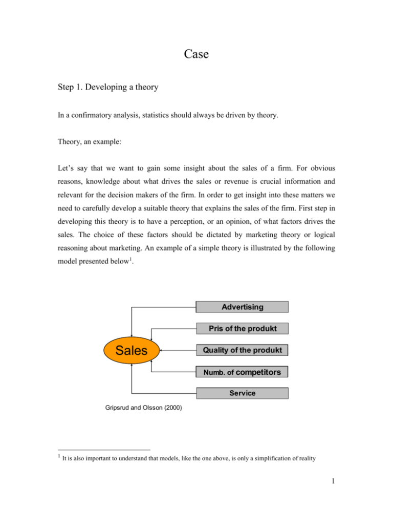
Case
Step 1. Developing a theory
In a confirmatory analysis, statistics should always be driven by theory.
Theory, an example:
Let’s say that we want to gain some insight about the sales of a firm. For obvious
reasons, knowledge about what drives the sales or revenue is crucial information and
relevant for the decision makers of the firm. In order to get insight into these matters we
need to carefully develop a suitable theory that explains the sales of the firm. First step in
developing this theory is to have a perception, or an opinion, of what factors drives the
sales. The choice of these factors should be dictated by marketing theory or logical
reasoning about marketing. An example of a simple theory is illustrated by the following
model presented below1.
Advertising
Pris of the produkt
Sales
Quality of the produkt
Numb. of competitors
Service
Gripsrud and Olsson (2000)
1
It is also important to understand that models, like the one above, is only a simplification of reality
1
It is quite reasonable to assume that factors, such as advertising, price of the product,
quality of the product, number of competitors and service, would have an impact on the
sales2. In this case these factors seem to be obvious choices. Even though the developed
theory appears to be quite plausible and reasonable, we would still want to confirm our
theory by some objective measurement. By objective measurement we often mean
statistical analysis. A well known and often used statistical tool is regression analysis,
which is one of the most applied tools in research.
A natural extension, and very important part, of the developing stage is to form, or
specify, a priori “before hand” opinion about how the different factors influence the
variable of interest, which in our specific case is sales. Using simple logic, one might
expect that advertising, quality, and service would have a positive impact on the sales,
while price and the number of competitors would have a negative impact.
Step 2. Model formulation
Before we are able to perform any statistical test, we need to formulate our theory
mathematically. A very general formulation of the model is of the form
Sales  f ( advertising, price of the product, quality of the product,
number of competitors, service)
This expression is not particularly informative and since we are using linear regression as
our primary tool, the model is expressed as the following linear relationship
Sales   0  1 advertising   2 price of the product +  3 quality of the product
+  4 number of competitors +  5 service,
2
Note that, in practice, some of these factors could be very difficult to measure.
2
where sales is the dependent variable (LHS of the equation) and advertising, price of the
product, quality of the product, number of competitors and service are independent
variables (RHS of the equation)3.  0 is referred to as the constant term, while
1 ,  2 ,.....,  5 is referred to as regression coefficients or regression parameters. By
definition, models are only simplifications of reality, and it is not possible to account for
all factors or variables that may have an impact on the dependent variable. For that
reason, we need to include a stochastic error term, denoted by epsilon, into the equation.
Sales   0  1 advertising   2 price of the product +  3 quality of the product
+  4 number of competitors +  5 service + 
The RHS of the equation is comprised of two parts. The first six terms is the
deterministic (explained) part, while  represents the stochastic (unexplained) part.
Interpretation of the model
The constant term  0 gives the value of the dependent variable when all the independent
variables are zero. Notice, that in most cases it can be difficult to give a meaningful
interpretation of the constant term. Unless one has a strong theoretical justification, the
constant term should always remain in the regression. If the constant term is removed
from the regression, critical assumptions underlying the OLS estimation technique might
be seriously violated, and the consequence could be that the statistical results become
highly unreliable. The regression coefficients ( 1 ,  2 ,.....,  5 ) measures how sensitive the
dependent variable is to a unit change in the associated independent variable. In other
words, if the absolute magnitude of  is large, only a small change in the independent
variable will have a significant impact on the dependent variable.
3
Independent variables are often referred to as predictor variables or explanatory variables.
3
Step 3. Model testing
An example:
In the following, an example of how to implement a simplified version of the model will
be given. The somewhat simpler model has this form
Sales   0  1 advertising +  2 quality + 
In this case Sales and advertising is measured in 1000 nkr and quality is an continuous
variable running from 0 to 10, where 0 indicates low product quality and 10 indicates
high product quality.
Before running the regression it is always advisable to perform a correlation analysis. The
correlation analysis will provide us with valuable information about the degree of covariation between the variables.
Correlations
ADVERTIS
SALES
QUALITY
Pears on Correlation
Sig. (2-tailed)
N
Pears on Correlation
Sig. (2-tailed)
N
Pears on Correlation
Sig. (2-tailed)
N
ADVERTIS
1
,
19
,664**
,002
19
,173
,480
19
SALES
QUALITY
,664**
,173
,002
,480
19
19
1
,252
,
,299
19
19
,252
1
,299
,
19
19
**. Correlation is s ignificant at the 0.01 level (2-tailed).
We clearly see that the relationship between advertising and Sales seems quite strong.
The correlation between these two variables equals 0.664. This number indicates that
there is a significant relationship between these two variables. The correlation between
the independent variables, advertising and quality, is relatively weak (0.0173). A strong
4
correlation between the independent variables could be an indication of problems with
multicollinarity in the data. Additionally, the correlation between quality and Sales is not
particularly strong either (0.299). At this point we have established that there is a positive
relationship between the dependent variable and the independent variables. These
observations are in line with the above suggested theory.
Running this regression model in SPSS, we get the following results
Model Summary
Model
1
R
R Square
,678 a
,460
Adjus ted
R Square
,392
Std. Error of
the Es timate
205,75668
a. Predictors : (Constant), QUALITY, ADVERTIS
ANOVAb
Model
1
Regress ion
Res idual
Total
Sum of
Squares
576141,8
677373,0
1253515
df
Mean Square
288070,887
42335,810
2
16
18
F
6,804
Sig.
,007 a
t
7,501
3,425
,757
Sig.
,000
,003
,460
a. Predictors : (Constant), QUALITY, ADVERTIS
b. Dependent Variable: SALES
Coefficientsa
Model
1
(Cons tant)
ADVERTIS
QUALITY
Uns tandardized
Coefficients
B
Std. Error
1074,899
143,300
19,711
5,754
11,464
15,135
Standardized
Coefficients
Beta
,639
,141
a. Dependent Variable: SALES
The statistical results should always be evaluated and discussed in light of theory and the
priori opinion formed in the step 1. (design stage). As can be seen from the tables, the
coefficient associated with advertising,  1 , equals 19.711. Note that the sign of this
coefficient is positive, meaning that an increase in advertising result in an increase in
sales. The interpretation is that, if we increase the level of marketing by 1000 nkr, sales
5
increases by 19.711 nkr. The same overall pattern and conclusions applies for the
variable quality. These observations are perfectly in line with our theory and priori
opinion.
Goodness of fit statistics
It is desirable to have measure of how well the regression model actually fits the data.
More specifically, it is desirable to have an answer to the question ‘how well does the
model containing the independent variables that was proposed actually explain the
variation in the dependent variable?’ We will use R 2 as a measure of how close the fitted
regression line is to all of the data points taken together. R 2 runs from 0 – 1, where 0
indicates independence (zero correlation) between the dependent variable and the
independent variable(s), while a value of 1 indicates perfect fit. Returning to the example,
if we take a look at the model summery we see that the adjusted value of R 2 equals
0.3924. This simply means that the two independent variables in our model explain about
40% of the variation in Sales. Even though this value might seem low, it is quite
reasonable.
Hypothesis testing
A crucial element of statistical analysis is hypothesis testing. More specifically we want
to test the individual regression coefficients as well as the entire model.
F-test
The F-test is used for testing multiple hypotheses
H 0 : 1   2  .......   k  0
H A : at least one  i  0
2
Note that we always use the adjusted value of R when the model contains more than one independent
variable in the model.
4
6
It can be seen from the alternative hypothesis ( H A ) that if only one regression coefficient
significantly deviates from zero, we reject the joint hypothesis ( H 0 ) , stating that all the
regression coefficients equals zero and statistically conclude that the model is adequate.
For our specific model we find that the p-value is less than 0.05 (0.007), which indicates
that at least one of the regression coefficients is significantly different from zero.
t-test
The t-test is used to test single hypothesis, i.e. hypothesis involving only one coefficient.
Normally we want to test the following hypothesis5
H0 :   0
HA :   0
In order to test this hypothesis we need to calculate the t-statistic. The formula for the tstatistic is
t

SE (  )
,
where SE (  ) is the standard deviation, which is a measure of the uncertainty associated
with the  -value. Given a significance level of 5%, the general rule is; if the absolute
value of the t-statistic is equal to or larger than 1.96 (gives a p-value < 0.05), we reject
the H 0 -hypothesis stating that the independent variable, associated with  , has no impact
on the dependent variable. We then adopt the alternative hypothesis ( H A ), stating that
the independent variable has a significant impact on the dependent variable. On the other
5
It could, however, be the case that our theory predicts that
 should have is a particular value.
7
hand, if the absolute value of the t-statistic is less than 1.96 (gives a p-value > 0.05), we
keep the H 0 -hypothesis.
From the table, containing the coefficients, we see that the t-statistic associated with
advertising equals 3.425. Since this value is significantly larger than 1.96, the p-value is
less than 0.05 (0.003). This means that we can statistically conclude that advertising has a
significant impact on sales. This confirms and increases the validity of our theory. The tstatistic can easily be calculated by hand from the information provided in the output
results
t-statistic 
19.711
 3.425
5.754
Note however that the t-statistic associated with the variable quality is less 1.96 and the
p-value is larger than 0.05 (0.46). By these statistics we cannot conclude that the  -value
is significantly different from zero. This conclusion is however in conflict with our theory
and it might be necessary to go back to step 1 and re-evaluate our theory. Another
explanation for this particular result could be that the variable, quality, fails to measure
the actual quality, then we have validity problem.
Given the evaluation so far, it might be a good idea to run a regression without the
variable quality.
Model Summary
Model
1
R
R Square
,664 a
,440
Adjus ted
R Square
,407
Std. Error of
the Es timate
203,16103
a. Predictors : (Constant), ADVERTIS
8
ANOVAb
Model
1
Regress ion
Res idual
Total
Sum of
Squares
551849,9
701664,9
1253515
df
1
17
18
Mean Square
551849,853
41274,405
F
13,370
Sig.
,002 a
a. Predictors : (Constant), ADVERTIS
b. Dependent Variable: SALES
Coefficientsa
Model
1
(Cons tant)
ADVERTIS
Uns tandardized
Coefficients
B
Std. Error
1100,651
137,452
20,464
5,597
Standardized
Coefficients
Beta
,664
t
8,008
3,657
Sig.
,000
,002
a. Dependent Variable: SALES
Even though we ha removed one variable from the analysis, the regression coefficient
and the t-statistic did not change much. Additionally, the value of R 2 is now 0.44, which
is somewhat higher than before. Notice that, since we are running a regression with a
single independent variable we do not use the adjusted value of R 2 as we did before.
These observations are a clear indication that the variable quality was an irrelevant
variable. The conclusion is that this model seems to be quite suitable and the best so far.
It is often the case that a simpler model is preferable, unless the results or theory suggests
otherwise.
9