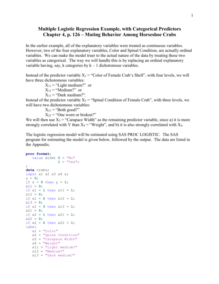
1
Multiple Logistic Regression Example, with Categorical Predictors
Chapter 4, p. 126 – Mating Behavior Among Horseshoe Crabs
In the earlier example, all of the explanatory variables were treated as continuous variables.
However, two of the four explanatory variables, Color and Spinal Condition, are actually ordinal
variables. We can make the model truer to the actual nature of the data by treating these two
variables as categorical. The way we will handle this is by replacing an ordinal explanatory
variable having, say, k categories by k – 1 dichotomous variables.
Instead of the predictor variable X1 = “Color of Female Crab’s Shell”, with four levels, we will
have three dichotomous variables:
X11 = “Light medium?” or
X12 = “Medium?” or
X13 = “Dark medium?”.
Instead of the predictor variable X2 = “Spinal Condition of Female Crab”, with three levels, we
will have two dichotomous variables:
X21 = “Both good?”
X22 = “One worn or broken?”
We will then use X3 = “Carapace Width” as the remaining predictor variable, since a) it is more
strongly correlated with Y than X4 = “Weight”, and b) it is also strongly correlated with X4.
The logistic regression model will be estimated using SAS PROC LOGISTIC. The SAS
program for estimating the model is given below, followed by the output. The data are listed in
the Appendix.
proc format;
value difmt 0 = "No"
1 = "Yes";
;
data crabs;
input x1 x2 x3 x4 s;
y = 0;
if s > 0 then y = 1;
x11 = 0;
if x1 = 1 then x11 = 1;
x12 = 0;
if x1 = 2 then x12 = 1;
x13 = 0;
if x1 = 3 then x13 = 1;
x21 = 0;
if x2 = 1 then x21 = 1;
x22 = 0;
if x2 = 2 then x22 = 1;
label
x1 = "Color"
x2 = "Spine Condition"
x3 = "Carapace Width"
x4 = "Weight"
x11 = "Light medium?"
x12 = "Medium?"
x13 = "Dark medium?"
2
x21 = "Both good?"
x22 = "One worn or broken?"
y = "Satellite Males?"
s = "No. of Satellite Males";
format y x11 x12 x13 x21 x22 difmt.;
cards;
The data set is listed in the earlier handout.
;
proc logistic;
model y (order=formatted event='Yes') = x11 x12 x13 x21 x22 x3 / covb;
title "Logistic regression of Satellite Presence";
title2 "vs. Several Explanatory Variables,";
title3 "Somc of which are Categorical";
;
proc corr;
var y x11 x12 x13 x21 x22 x3;
title "Correlations Among All Variables";
title2 "Including Number of Satellite Males";
;
run;
3
SAS Output for Full Model, Including All Explanatory Variables:
Logistic regression of Satellite Presence
6
vs. Several Explanatory Variables,
Somc of which are Categorical
11:31 Wednesday, November 5, 2008
The LOGISTIC Procedure
Model Information
Data Set
WORK.CRABS
Response Variable
y
Satellite Males?
Number of Response Levels
2
Model
binary logit
Optimization Technique
Fisher's scoring
Number of Observations Read
173
Number of Observations Used
173
Response Profile
Ordered
Total
Value
y
Frequency
1
No
62
2
Yes
111
Probability modeled is y='Yes'.
Model Convergence Status
Convergence criterion (GCONV=1E-8) satisfied.
Model Fit Statistics
Intercept
Intercept
and
Criterion
Only
Covariates
AIC
227.759
200.612
SC
230.912
222.685
-2 Log L
225.759
186.612
Logistic regression of Satellite Presence
7
vs. Several Explanatory Variables,
Somc of which are Categorical
11:31 Wednesday, November 5, 2008
The LOGISTIC Procedure
Testing Global Null Hypothesis: BETA=0
Test
Chi-Square
DF
Pr > ChiSq
Likelihood Ratio
39.1466
6
<.0001
Score
35.3481
6
<.0001
Wald
28.4898
6
<.0001
Parameter
Intercept
x11
x12
x13
x21
x22
x3
Analysis of Maximum Likelihood Estimates
Standard
Wald
DF
Estimate
Error
Chi-Square
1
-12.3908
2.8194
19.3153
1
1.6683
0.9329
3.1985
1
1.5249
0.5672
7.2285
1
1.1443
0.5933
3.7199
1
-0.3770
0.5019
0.5643
1
-0.4348
0.6254
0.4834
1
0.4562
0.1078
17.9141
Effect
x11
x12
x13
x21
x22
x3
Odds Ratio Estimates
Point
95% Wald
Estimate
Confidence Limits
5.303
0.852
33.006
4.595
1.512
13.966
3.140
0.982
10.045
0.686
0.256
1.834
0.647
0.190
2.205
1.578
1.278
1.949
Pr > ChiSq
<.0001
0.0737
0.0072
0.0538
0.4525
0.4869
<.0001
4
Association of Predicted Probabilities and Observed Responses
Percent Concordant
77.3
Somers' D
0.549
Percent Discordant
22.4
Gamma
0.551
Percent Tied
0.3
Tau-a
0.254
Pairs
6882
c
0.775
Parameter
Intercept
x11
x12
x13
x21
x22
x3
7
Intercept
7.948753
0.019563
-0.16101
-0.2992
0.049164
-0.36215
-0.29929
Variables:
Variable
y
x11
x12
x13
x21
x22
x3
Logistic regression of Satellite Presence
8
vs. Several Explanatory Variables,
Somc of which are Categorical
11:31 Wednesday, November 5, 2008
The LOGISTIC Procedure
Estimated Covariance Matrix
x11
x12
x13
x21
x22
x3
0.019563
-0.16101
-0.2992
0.049164
-0.36215
-0.29929
0.870212
0.293014
0.252517
-0.17261
-0.14623
-0.00969
0.293014
0.321701
0.244704
-0.06079
-0.06118
-0.0029
0.252517
0.244704
0.351987
-0.01315
-0.03011
0.00237
-0.17261
-0.06079
-0.01315
0.251913
0.074371
-0.00236
-0.14623
-0.06118
-0.03011
0.074371
0.39115
0.013802
-0.00969
-0.0029
0.00237
-0.00236
0.013802
0.01162
y
N
173
173
173
173
173
173
173
Correlations Among All Variables
9
Including Number of Satellite Males
11:31 Wednesday, November 5, 2008
The CORR Procedure
x11
x12
x13
x21
x22
x3
Simple Statistics
Mean
Std Dev
Sum
Minimum
Maximum
0.64162
0.48092
111.00000
0
1.00000
0.06936
0.25481
12.00000
0
1.00000
0.54913
0.49902
95.00000
0
1.00000
0.25434
0.43675
44.00000
0
1.00000
0.21387
0.41123
37.00000
0
1.00000
0.08671
0.28222
15.00000
0
1.00000
26.29884
2.10906
4550
21.00000
33.50000
Simple Statistics
Variable
Label
y
Satellite Males?
x11
Light medium?
x12
Medium?
x13
Dark medium?
x21
Both good?
x22
One worn or broken?
x3
Carapace Width
Pearson Correlation Coefficients, N = 173
Prob > |r| under H0: Rho=0
y
Satellite Males?
x11
Light medium?
x12
Medium?
x13
Dark medium?
x21
Both good?
x22
One worn or broken?
x3
Carapace Width
y
1.00000
0.06171
0.4200
0.19493
0.0102
-0.06176
0.4195
0.06644
0.3851
-0.11242
0.1409
0.40141
<.0001
x11
0.06171
0.4200
1.00000
-0.30130
<.0001
-0.15944
0.0361
0.35696
<.0001
0.07758
0.3103
0.08670
0.2567
x12
0.19493
0.0102
-0.30130
<.0001
1.00000
-0.64453
<.0001
0.10432
0.1720
-0.00978
0.8983
0.21273
0.0050
x13
-0.06176
0.4195
-0.15944
0.0361
-0.64453
<.0001
1.00000
-0.20751
0.0062
0.00872
0.9093
-0.15242
0.0453
x21
0.06644
0.3851
0.35696
<.0001
0.10432
0.1720
-0.20751
0.0062
1.00000
-0.16071
0.0347
0.20139
0.0079
x22
-0.11242
0.1409
0.07758
0.3103
-0.00978
0.8983
0.00872
0.9093
-0.16071
0.0347
1.00000
-0.23035
0.0023
x3
0.40141
<.0001
0.08670
0.2567
0.21273
0.0050
-0.15242
0.0453
0.20139
0.0079
-0.23035
0.0023
1.00000
5
Next, we want to find a subset of these variables that works in our model, since it is possible that
some of the dichotomous explanatory variables do not contribute to the explanatory power of the
model. We look at the correlations (phi coefficients) between Y and each of the dichotomous
variables to choose a likely subset of variables to eliminate. The variables that are least strongly
correlated with Y are X11, X13, and X21. We will fit a model without these variables, and then
test whether they may be eliminated by comparing the two models. The output for the full model
is given above. The output for the reduced model is listed below.
SAS Output for Reduced Model:
Logistic regression of Satellite Presence
1
vs. Several Explanatory Variables,
Somc of which are Categorical
Reduced Model
14:58 Wednesday, November 5, 2008
The LOGISTIC Procedure
Model Information
Data Set
WORK.CRABS
Response Variable
y
Satellite Males?
Number of Response Levels
2
Model
binary logit
Optimization Technique
Fisher's scoring
Number of Observations Read
173
Number of Observations Used
173
Response Profile
Ordered
Total
Value
y
Frequency
1
No
62
2
Yes
111
Probability modeled is y='Yes'.
Model Convergence Status
Convergence criterion (GCONV=1E-8) satisfied.
Model Fit Statistics
Intercept
Intercept
and
Criterion
Only
Covariates
AIC
227.759
199.697
SC
230.912
212.310
-2 Log L
225.759
191.697
Logistic regression of Satellite Presence
2
vs. Several Explanatory Variables,
Somc of which are Categorical
Reduced Model
14:58 Wednesday, November 5, 2008
The LOGISTIC Procedure
Testing Global Null Hypothesis: BETA=0
Test
Chi-Square
DF
Pr > ChiSq
Likelihood Ratio
34.0617
3
<.0001
Score
30.1587
3
<.0001
Wald
25.3813
3
<.0001
Parameter
Intercept
x12
x22
x3
Analysis of Maximum Likelihood Estimates
Standard
Wald
DF
Estimate
Error
Chi-Square
1
-12.0239
2.7321
19.3692
1
0.5823
0.3525
2.7284
1
-0.1463
0.5960
0.0603
1
0.4736
0.1055
20.1555
Odds Ratio Estimates
Pr > ChiSq
<.0001
0.0986
0.8061
<.0001
6
Effect
x12
x22
x3
Point
Estimate
1.790
0.864
1.606
95% Wald
Confidence Limits
0.897
3.572
0.269
2.778
1.306
1.975
Association of Predicted Probabilities and Observed Responses
Percent Concordant
74.6
Somers' D
0.499
Percent Discordant
24.7
Gamma
0.502
Percent Tied
0.6
Tau-a
0.231
Pairs
6882
c
0.749
7
Parameter
Intercept
x12
x22
x3
Logistic regression of Satellite Presence
3
vs. Several Explanatory Variables,
Somc of which are Categorical
Reduced Model
14:58 Wednesday, November 5, 2008
The LOGISTIC Procedure
Estimated Covariance Matrix
Intercept
x12
x22
x3
7.46416
0.010161
-0.37749
-0.28698
0.010161
0.124258
-0.01469
-0.00273
-0.37749
-0.01469
0.355191
0.013524
-0.28698
-0.00273
0.013524
0.011128
Now we want to compare the full model and the reduced model to see whether the reduced
model is adequate.
Step 1: H0: 11  13   21  0
v.
HA: Not all three are 0.
Step 2: We have n  173 ,  = 0.05.
Step 3: The test statistic is the Likelihood Ratio chi-square statistic G 2  2l 0  l1  , where l1 is
the maximum of the log-likelihood function for the reduced model, and l 0 is the maximum of the
log-likelihood function for the full model. Under the null hypothesis, the statistic G 2 has a chisquare distribution with d.f. = 3, since we are hypothesizing that we may eliminate three of the
parameters from the full model.
Step 4: We will reject the null hypothesis if G2 >  32, 0.05  7.81 .
Step 5: From the two outputs, we find G2 = 191.697 – 186.612 = 5.085.
Step 6: We fail to reject the null hypothesis at the 0.05 level of significance. We do not have
sufficient evidence to conclude that the variables X11, X13, and X21 provide additional
explanatory power to predict the value of Y.
Thus, we choose the reduced model to explain Y, using the predictors X12 = “Medium Color?”,
X22 = “One worn or broken?”, and X = “Carapace Width.” However, we then may want to test
whether one of the dichotomous variables is extraneous. We choose X22, since it is not
substantially correlated with Y. We use the above model as the full model, and estimate a
reduced model with the additional predictor eliminated.
Logistic regression of Satellite Presence
1
vs. Several Explanatory Variables,
Somc of which are Categorical
15:18 Wednesday, November 5, 2008
The LOGISTIC Procedure
Model Information
Data Set
WORK.CRABS
Response Variable
y
Satellite Males?
Number of Response Levels
2
Model
binary logit
Optimization Technique
Fisher's scoring
Number of Observations Read
173
Number of Observations Used
173
8
Response Profile
Ordered
Total
Value
y
Frequency
1
No
62
2
Yes
111
Probability modeled is y='Yes'.
Model Convergence Status
Convergence criterion (GCONV=1E-8) satisfied.
Model Fit Statistics
Intercept
Intercept
and
Criterion
Only
Covariates
AIC
227.759
197.757
SC
230.912
207.217
-2 Log L
225.759
191.757
Logistic regression of Satellite Presence
2
vs. Several Explanatory Variables,
Somc of which are Categorical
15:18 Wednesday, November 5, 2008
The LOGISTIC Procedure
Testing Global Null Hypothesis: BETA=0
Test
Chi-Square
DF
Pr > ChiSq
Likelihood Ratio
34.0014
2
<.0001
Score
30.0492
2
<.0001
Wald
25.2770
2
<.0001
Parameter
Intercept
x12
x3
Analysis of Maximum Likelihood Estimates
Standard
Wald
DF
Estimate
Error
Chi-Square
1
-12.1827
2.6617
20.9495
1
0.5763
0.3516
2.6873
1
0.4793
0.1032
21.5756
Effect
x12
x3
Pr > ChiSq
<.0001
0.1011
<.0001
Odds Ratio Estimates
Point
95% Wald
Estimate
Confidence Limits
1.779
0.893
3.544
1.615
1.319
1.977
Association of Predicted Probabilities and Observed Responses
Percent Concordant
74.4
Somers' D
0.501
Percent Discordant
24.3
Gamma
0.508
Percent Tied
1.3
Tau-a
0.232
Pairs
6882
c
0.751
Parameter
Intercept
x12
x3
Estimated Covariance Matrix
Intercept
x12
7.084613
-0.00481
-0.00481
0.123591
-0.27346
-0.0022
x3
-0.27346
-0.0022
0.010647
9
Step 1: H0:  22  0
v.
HA:  22  0 .
Step 2: We have n  173 ,  = 0.05.
Step 3: The test statistic is the Likelihood Ratio chi-square statistic G 2  2l 0  l1  , where l1 is
the maximum of the log-likelihood function for the reduced model, and l 0 is the maximum of the
log-likelihood function for the full model. Under the null hypothesis, the statistic G 2 has a chisquare distribution with d.f. = 1, since we are hypothesizing that we may eliminate one of the
parameters from the full model.
Step 4: We will reject the null hypothesis if G2 > 12, 0.05  3.84 .
Step 5: From the two outputs, we find G2 = 191.757 – 191.697 = 0.06.
Step 6: We fail to reject the null hypothesis at the 0.05 level of significance. We do not have
sufficient evidence to conclude that the variable X22 provides additional explanatory power to
predict the value of Y.
Thus our final model for predicting the presence of satellite males includes whether the color of
the female crab’s shell is medium, and the width of the carapace of the female crab. (We could
compare this model with the model containing only the carapace width, but we would find that
the two variables together do provide better explanatory power.)