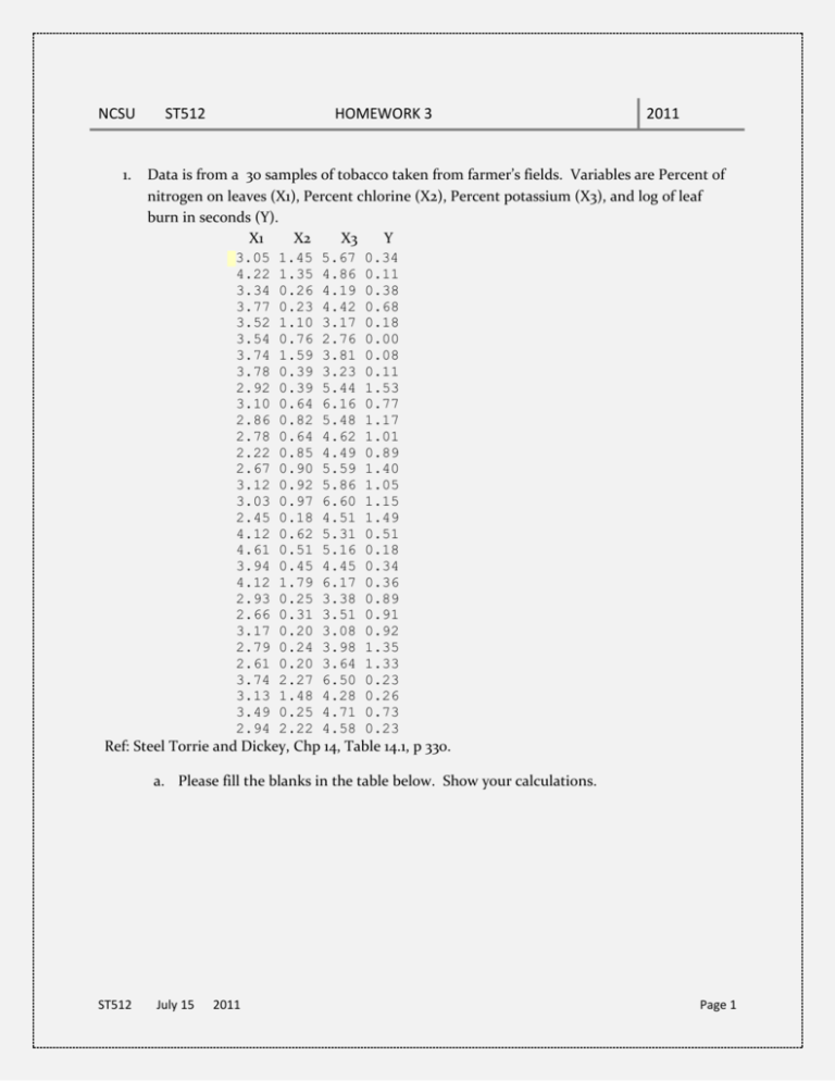
NCSU
ST512
HOMEWORK 3
2011
1.
Data is from a 30 samples of tobacco taken from farmer’s fields. Variables are Percent of
nitrogen on leaves (X1), Percent chlorine (X2), Percent potassium (X3), and log of leaf
burn in seconds (Y).
X1
X2
X3
Y
3.05 1.45 5.67 0.34
4.22 1.35 4.86 0.11
3.34 0.26 4.19 0.38
3.77 0.23 4.42 0.68
3.52 1.10 3.17 0.18
3.54 0.76 2.76 0.00
3.74 1.59 3.81 0.08
3.78 0.39 3.23 0.11
2.92 0.39 5.44 1.53
3.10 0.64 6.16 0.77
2.86 0.82 5.48 1.17
2.78 0.64 4.62 1.01
2.22 0.85 4.49 0.89
2.67 0.90 5.59 1.40
3.12 0.92 5.86 1.05
3.03 0.97 6.60 1.15
2.45 0.18 4.51 1.49
4.12 0.62 5.31 0.51
4.61 0.51 5.16 0.18
3.94 0.45 4.45 0.34
4.12 1.79 6.17 0.36
2.93 0.25 3.38 0.89
2.66 0.31 3.51 0.91
3.17 0.20 3.08 0.92
2.79 0.24 3.98 1.35
2.61 0.20 3.64 1.33
3.74 2.27 6.50 0.23
3.13 1.48 4.28 0.26
3.49 0.25 4.71 0.73
2.94 2.22 4.58 0.23
Ref: Steel Torrie and Dickey, Chp 14, Table 14.1, p 330.
a. Please fill the blanks in the table below. Show your calculations.
ST512
July 15
2011
Page 1
Parameter Estimates
Variable
Parameter Standard
DF
Estimate
Error t Value Pr > |t| Type I SS Type II SS
Intercept
1
2.56226
0.39767
6.44 <.0001
x1
1
-0.75685
0.11137
-6.80 <.0001
x2
1
-1.45070
0.41538
-3.49 0.0018
x4
1
0.29941
0.12141
2.47 0.0209
x3
1
0.20686
0.03718
5.56 <.0001
14.11788
1.58242
 
b. Show Type I SS o  ny 2
c. Write the multiple regression equation.
d. Test the hypothesis H o : 3  0
vs
H o : 3  0 Use  =0.05
e. Test the hypothesis H o :  4  0
vs
H o :  4  0 Use  =0.05
f.
Test the hypothesis H o : 2  3  0
vs
H o : not all i  0
Use  =0.05
g. A friend asked you to compute the regression equation that show the effect of X1 and
X2 on Y when X3 is kept constant at its average value. You need to show her that the
coefficient of X2 depends on X1. Find out the regression coefficient for X2 when X1 =
3, and also for X1= 4.
h. Should we expect the slope for X2 become positive? If yes, at what value of X1?
1 model y= x1 x2 x3
pred
2.84
1.51
4.61
0.18
3.81
x1
-1.16
2.27
3.02
1.57
x2
0.88
0.18
2.22
2) A poultry Scientist was studying a the creation of a new diet. A food additive added to the
standard basal diet. He have varying amount of the additive: 0 20 40 60 80 100, and each of
the 6 diets were assigned to 10 chickens. 5 chickens in each group received additionally 400
ppm of copper while the remaining 5 chickens received no copper. At the end of the study the
ST512
July 15
2011
Page 2
feed efficiency ratio (feed consumed(gm) to weight gain (gm) was obtained for the sixty
chickens. Data is attached.
a. Fit the following two regression equations
Model 1: y   o  1 x1   2 x12  3 x13  e
Model 2 : y   o  1 x1   2 x12  3 x2  e
Model 3 : y   o  1 x1   2 x12  3 x2   4 x1 x2  5 x12 x2  e
Y= Feed Efficiency ratio,
X1 = Amount of feed additive,
X2 = Amount of copper placed in feed.
b. Which models appears to provide the better fitting to the data. Justify your answer.
c. Display the predicted equation for the best fitting model.
Ref” Ott and Longnecker, Ex. 14.14 , p 735
Data
Cu Additive FeedEffRatio
0
0
0
0
0
400
400
400
400
400
0
0
0
0
0
400
400
400
400
400
0
0
0
0
0
400
400
400
400
400
ST512
0
0
0
0
0
0
0
0
0
0
20
20
20
20
20
20
20
20
20
20
40
40
40
40
40
40
40
40
40
40
July 15
1.3
1.35
1.44
1.52
1.56
1.61
1.48
1.56
1.45
1.14
2.17
2.11
2.08
2.13
2.22
2.29
2.33
2.24
2.16
2.21
2.3
2.34
2.2
2.38
2.48
2.44
2.37
2.43
2.37
2.41
2011
Page 3
0
0
0
0
0
400
400
400
400
400
0
0
0
0
0
400
400
400
400
400
0
0
0
0
0
400
400
400
400
400
ST512
60
60
60
60
60
60
60
60
60
60
80
80
80
80
80
80
80
80
80
80
100
100
100
100
100
100
100
100
100
100
July 15
2.47
2.51
2.79
2.4
2.55
2.67
2.5
2.55
2.6
2.49
3.31
3.17
3.24
3.21
3.35
3.38
3.42
3.36
3.25
3.51
4.92
3.87
4.81
4.88
5.06
5.09
4.97
4.95
4.59
4.76
2011
Page 4