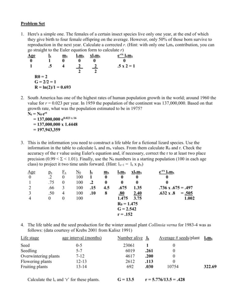
Problem Set
1. Here's a simple one. The females of a certain insect species live only one year, at the end of which
they give birth to four female offspring on the average. However, only 50% of those born survive to
reproduction in the next year. Calculate a corrected r. (Hint: with only one lxmx contribution, you can
go straight to the Euler equation form to calculate r)
Age
lx
mx
lxmx xlxmx
e-rx lxmx
0
1
0
0
0
0
1
.5
4
_2_
2
.5 x 2 = 1
2
2
R0 = 2
G = 2/2 = 1
R = ln(2)/1 = 0.693
2. South America has one of the highest rates of human population growth in the world; around 1960 the
value for r = 0.023 per year. In 1959 the population of the continent was 137,000,000. Based on that
growth rate, what was the population estimated to be in 1975?
Nt = N0 ert
= 137,000,000 e0.023 x 16
= 137,000,000 x 1.4448
= 197,943,359
3. This is the information you need to construct a life table for a fictional lizard species. Use the
information in the table to calculate lx and mx values. From them calculate R0 and r. Check the
accuracy of the r value using Euler's equation and, if necessary, correct the r to at least two place
precision (0.99 <  < 1.01). Finally, use the N0 numbers in a starting population (100 in each age
class) to project it two time units forward. (Hint: lx+1 = lx x px)
Age
0
1
2
3
4
px
.2
.75
.66
.50
0
Fx
0
0
3
4
0
N0
100
100
100
100
100
lx
1
.2
.15
.10
mx
0
0
4.5
8
e-rx lxmx
0
0
.736 x .675 = .497
.632 x .8 = .505
1.002
lxmx xlxmx
0
0
0
0
.675
1.35
.80
2.40
1.475 3.75
R0 = 1.475
G = 2.542
r = .152
4. The life table and the seed production for the winter annual plant Collinsia verna for 1983-4 was as
follows: (data courtesy of Krebs 2001 from Kalisz 1991)
Life stage
Seed
Seedling
Overwintering plants
Flowering plants
Fruiting plants
age interval (months)
0-5
5-7
7-12
12-13
13-14
Calculate the lx and ‘r’ for these plants.
Number alive lx
23061
6019
4617
2612
692
G = 13.5
1
.261
.200
.113
.030
Average # seeds/plant
0
0
0
0
10754
r = 5.776/13.5 = .428
lxmx
322.69
5. You survey an annual insect and find 5000 females per acre. One year later you census the population
and find 6000 females per acre. What is the net replacement rate, R0, this population? What size will
the population be three years from the original census if the population continues to grow at the same
rate? How many years will it take for the population to reach 100,000?
R0 = 6000/5000 = 1.2
N3 = N0 x R03 = 5000 x 1.728 = 8640
100,000 = 5000 x 1.2n
n = 16.46
6 In 1981, the world human population was 4.5 billion. The birth rate was 28 per thousand (=.028 per
capita) and the death rate was 11 per thousand (= 0.011). Thus the r-value was 0.017. Using these
figures, project the population for 20 years to 2001. Compare this projection to the actual human
population of 6.1 billion in 2001. Now project the population 119 years to 2100. What is the projected
human population in 2100 based on 1981 data? How does this compare to the 11 billion projected by
the UN?
Nt = N0 ert
= 4.5 x e.017 x 20 = 4.5 x 1.4049 = 6.322 (in billions) in 2001
The population in 2001 was smaller than the exponential growth prediction
N2100 = N1981 e .017 x 119 = 4.5 x 7.56 = 34.02 (in billions)
Population growth projected by the UN shows a great decrease in rate compared to the
exponential prediction based on rate in 1981.
7
What are R0 and the gross reproductive rate for the following population?
Age class (x)
0
1
2
3
4
5
l(x)
m(x)
lxmx
1.0
0.8
0.6
0.4
0.2
0
0
1
2.0
2.1
2.6
0
7.7 = GRR
0
0.8
1.2
.84
.52
0
3.36 = R0
8. For the information in the following life table, calculate the gross and net reproductive rate, and also
the intrinsic rate of increase.
Age class (x)
0
1
2
3
l(x)
1.0
0.6
0.3
0
m(x)
lxmx
xlxmx
0
0
0
2
1.2
1.2
2
0.6
1.2
0__ 0
0
Σ4
1.8
2.4
Gross Reproductive Rate = 4
Net Reproductive Rate = 1.8
r = ln (R0)/T = ln(1.8)/[2.4/1.8] = .587/1.333 = 0.441
9. Draw a survivorship curve for each of two populations of the same species. One cohort is started at
high density; the other cohort is started at low density. Mortality in this species shows density
dependence. Label axes, provide arbitrary scales, and label your curves.
10. A field survey of bruchid beetles revealed a dense population of the beetle on one species of Acacia
tree and very few beetles on a second species of Acacia. Samples of the second Acacia were brought
into the laboratory and a cohort of beetle eggs was placed on the leaves, from which the following life
table for the beetle was developed:
Age class (x) l(x)
0
1
2
3
4
5
6
7
1.0
0.9
0.7
0.6
0.4
0.3
0.15
0
m(x)
l(x)m(x)
0
0
0.1
0.2
0.3
0.1
0.1
---
0
0
.07
.12
.12
.03
.015
 = .355
Does the life table provide any clues about the rarity of the beetle on the second species of Acacia?
Gross reproductive rate is only 0.8
Net reproductive rate is 0.355, the population would decline rapidly
11. Here is hypothetical field survey data for a population of pond snails, Helisoma trivolvis. The values
collected are S(x), the number of snails from an initial, introduced cohort released in the pond, and
b(x), the mean number of egg sacks produced by a snail (they are hermaphroditic). Egg sacks each
contain 10 fertilized eggs.
Age in years (x)
S(x)
b(x)
0
1
2
3
500
400
40
0
0.0
0.6
3.5
----
Complete the life table by calculating l(x), p(x), R0, G and an initial estimate of r. Use Euler’s
equation to correct r so that 0.99 < Σe-rx l(x)m(x) < 1.01.
Age
0
1
2
3
N(x)
500
400
40
0
l(x)
1.0
0.8
0.08
0
p(x)
0.8
0.1
0
---
b(x)
0
6
3.5
---
l(x)m(x)
0
4.8
2.8
---=7.6
e-rxl(x)m(x)
0
1.092
.145
xl(x)m(x)
0
4.8
5.6
---10.4
1.237
R0 = 7.6
G = 10.4/7.6=1.368
r = ln 7.6/1.368=1.48
Initial attempt gives a sum too large. Make r larger, try 1.6, then …
1.6
1.7
1.65
1.675
1.6725
e-rxl(x)m(x)
e-rxl(x)m(x)
0
0
0
0
0
.969
.876
.921
.899
.901
.114
.093
.103
.098
.098
 = 1.083
.969
1.024
.997
.999
12. The following schedule of births and deaths is for a population that triples each generation. What is the
value for m4? Show your calculations!
Age class (x)
0
1
2
3
4
5
l(x)
1.0
0.7
0.5
0.4
0.2
0
m(x)
0
2.0
1.8
1.25
?
lxmx
0
1.4
0.9
0.5
0.2
3.0
m4 = 1
13. The giant lobelia, Lobelia deckenii, on Mount Kenya produces on average 250,000 seeds. Average
adult survivorship is 0.984 per year. Plants do not begin setting seed until they are ~50 years old. What
must the survivorship of seeds be to produce a stable population (λ = 1)?
p1 - p50  .98450
250,000 x .98450 x seed survivorship = 1
111,608 x seed survivorship = 1
Seed survivorship = .00000896
14. Determine the doubling times for the following human populations (realized instantaneous rates of
increase from U.N. data for 1999):
Country
Realized instantaneous
Rate of population increase
Ghana
0.029
South Africa
0.016
Canada
0.004
United Kingdom
0.002
Argentina
0.012
Russia
-0.005
Doubling time
23.90
43.31
173.25
346.5
57.75
decreasing, no doubling time
15. This problem is stolen from Krebs (2001) because it presents an important view of human population
growth. If the human population instantly adopted zero population growth (R0 = 1), the population
would continue to grow until it reached a stationary age distribution. Keyfitz (1971) showed that such
a population would continue to increase by demographic momentum, as follows:
Q
. 
be  R0  10


ra  R0 
Where Q = finite rate of population change (1.0 = no change)
b = crude birth rate per 1000 persons
e = life expectancy at birth in years
r = current rate of natural increase per 1000 persons
a = average age at first reproduction in years
A human population growing at these rates would increase Q times before it reached equilibrium. In
1998 the parameters for the global population were b =28, e = 61, r = 17,
a = 25, and R0 = 1.77. If
the human population is now ~7 billion, what is the value of Q based on those 1988 parameters, and
how large would the population be by the time a stationary age distribution was reached?
Q = ([28 x 61]/[17 x 25]) x [.77/1.77]
= 1.748
Population at equilibrium = 7,000,000,000 x 1.748
= 12.236 billion
16. Both abiotic and biotic factors influence the birth and death rates of populations and species. Choose a
species common in this area and make a list of the abiotic and biotic factors that are potentially
important in regulating the local population of that species.
There is no single answer to this question.
17. A population of insects triples every year. Initially there were 40 insects. How many insects would
there be after 4 years? How many insects would there be after 27 years? (Write the answer to this
question as an equation, as well as the solution.) Assume that the habitat of this insect degraded when
the population size reached 100, causing a decrease in  from 3 to 0.75. How many insects would
there be 3 years after this habitat change?
N4 = 40 x 34 = 3240
N27 = 40 x 327 = 3.05 x 1014
N3 = 100 x .753= 42.1