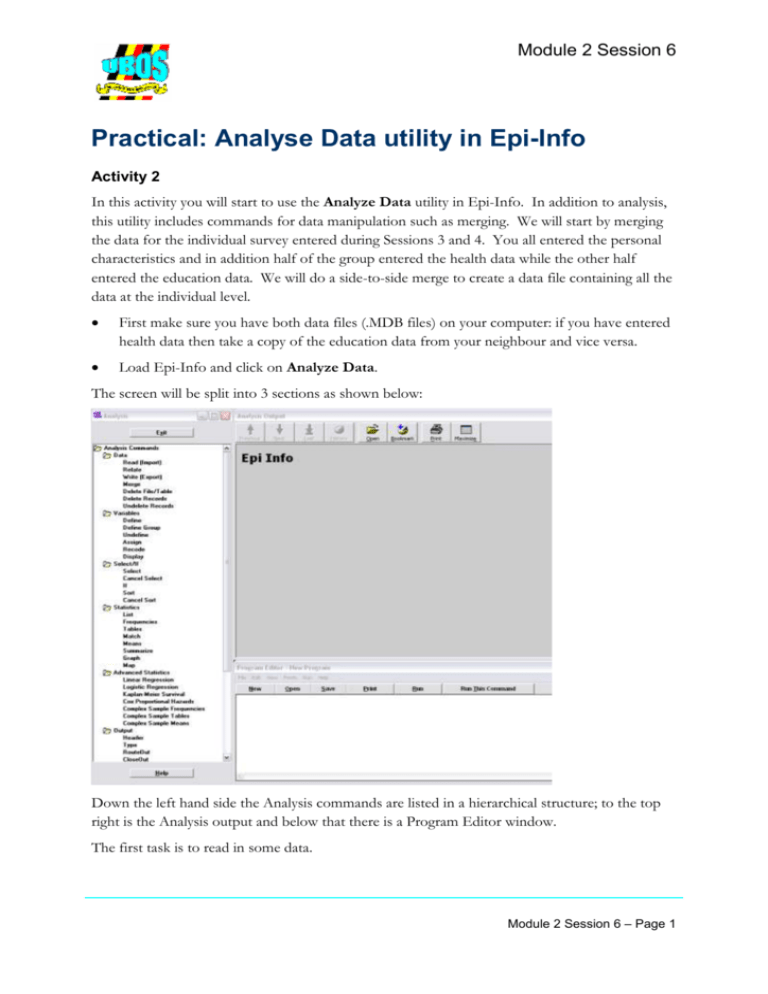
Module 2 Session 6
Practical: Analyse Data utility in Epi-Info
Activity 2
In this activity you will start to use the Analyze Data utility in Epi-Info. In addition to analysis,
this utility includes commands for data manipulation such as merging. We will start by merging
the data for the individual survey entered during Sessions 3 and 4. You all entered the personal
characteristics and in addition half of the group entered the health data while the other half
entered the education data. We will do a side-to-side merge to create a data file containing all the
data at the individual level.

First make sure you have both data files (.MDB files) on your computer: if you have entered
health data then take a copy of the education data from your neighbour and vice versa.

Load Epi-Info and click on Analyze Data.
The screen will be split into 3 sections as shown below:
Down the left hand side the Analysis commands are listed in a hierarchical structure; to the top
right is the Analysis output and below that there is a Program Editor window.
The first task is to read in some data.
Module 2 Session 6 – Page 1
Module 2 Session 6

In the command list click on Read (Import). The following dialog box appears:
The Current Project is the database file (.MDB) which is the default source of data and the
destination for output tables of statistical functions. At this point you have a choice:
1. You can either save your output in the same project file as your data, or
2. You can save any output to a different project, linking in the data as and when needed.
There are pros and cons for each approach but for the purposes of this practical we will choose
option 1; you can experiment with option 2 in your own time.

If the current project is not showing the correct name of your project file then click Change
Project and select the correct file.

The Data Source should be the same as the current project – this is the file you created in
Session 3.

The only view should be viewIndividuals so select this view and click OK.

To see these data in a grid format (rows and columns) choose the List command and in the
dialog box tick the check box for All – click OK
Module 2 Session 6 – Page 2
Module 2 Session 6
The table shows the 20 records you entered. It will have the household ID (HHID) and the
individual ID (PID). You should also see the 8 variables from section 2 of the questionnaire and
either the 7 variables from the health section or the 6 variables from the education section.
Your next task is to add the data that you didn’t enter in Session 4. This will be in the file from
your neighbour. This is a side-to-side merge so we use the Relate command.

Click on Relate in the command list.

Change the Data Source to match the name of the file from your neighbour

This file should also have just the one view called viewIndividuals so select this view.

As the Key enter HHID::HHID AND PID::PID – the key identifier for records in this
dataset is the combination of the household ID and the individual ID. Your dialog box
should now resemble that shown below:

Click OK
Module 2 Session 6 – Page 3
Module 2 Session 6
You now have a choice of making a temporary link in the current project, which means these
data will only be linked to the project while you remain in the Analyze Data utility, or you can
create a permanent link by entering a new table name. We will use a temporary link.

Click OK
Note that as you run each command, the syntax automatically appears in the Program Editor
Window from where it can be saved as a Program file. You can also select commands from the
Program Editor Window and rerun them.

Rerun the command to view the data by selecting LIST * GRIDTABLE and clicking Run
This Command.

Use the horizontal scroll bar to see what variables you now have in your dataset. What do
you notice?
You should notice that the variables from Section 2 and the key variables have been repeated.
The duplicate variables all have the suffix of “1” in their names. Ideally we don’t want to include
these duplicate variables in our dataset. On the Relate command there is not an option to select
which variables to include. Therefore to save the complete dataset without duplicate variables we
will use the Write command.

Choose Write (Export)

Uncheck the All box as this would output all variables.

In the variables list select HHID and PID together with the 8 variables from Section 2
(S2Q2 to S2Q9), the 7 variables from Section 3 (S3Q2 to S3Q8) and the 6 variables from
Section 4 (S4Q2 to S4Q7).

As the Data Table enter IndividualsAll or any other appropriate name to indicate that this
table contains all sections of the individual’s data. The File Name should be the same as
the current project.
Module 2 Session 6 – Page 4
Module 2 Session 6
Note: the Write command can be used to export data in a variety of formats. We will explore
this feature later when we export data to be used in another package.
In the next practical session we will use these merged data to produce some simple tables and
graphs.
Activity 4

If you have come out of the Analyze data utility then go back into it and load the data you
saved during the last part of the practical – IndividualsAll.

Produce frequency tables for variables S2Q2, S2Q4, S2Q5 and S2Q7 using the command
Frequencies.
Module 2 Session 6 – Page 5
Module 2 Session 6
1. How many individuals from our sample have not been in the household for the
last 12 months? ___________
2. What percentage of the sample are female? ___________
3. What percentage of the sample are married? __________
How easy is it to answer these questions by just looking at the results? The chances are you
probably had to clarify things with your neighbour or refer back to the questionnaire. To make
the results easier to understand we will do some recoding.

Use the Define command to define a new variable for marital status. Make this a Text
variable called Marital_Status.

Then use the Recode command to recode variable S2Q7 into this new variable. Set the
recoding as follows:
Module 2 Session 6 – Page 6
Module 2 Session 6

In the same way create a new text variable called Relationship_To_Head and recode the
current variable S2Q4 into it using the coding system from the questionnaire.

Now rerun the frequencies this time using the variables Marital_Status and
Relationship_To_Head. Are the results now clearer?
Copy and Paste Output
In Session 10 of this module you will be putting together a report on this set of data. It is a good
idea to include output from your analyses in your report. To help build your report we will copy
and paste the frequency tables into a new Word document that you will later turn into your
report.

Leaving Epi-Info open and running, open a new blank document in Word.

In Epi-Info scroll back through the output window and, using the mouse, select the
frequency table for the sex variable as shown below:

Use <Ctrl-C> to copy this table to the clipboard.

Go into your new Word document and use <Ctrl-V> to paste the table.

Repeat this process for the Marital_Status and Relationship_To_Head frequency tables.

Save the Word file giving it a suitable name such as “Household Survey Results”. Do not
close the file as we will add to it as we go through this practical session.
Cross-tabulations
Your next task is to produce a cross-tabulation of relationship against sex.

Use the Tables command to create a cross-tabulation of Relationship_To_Head against
sex (S2Q5).
Module 2 Session 6 – Page 7
Module 2 Session 6
1. What percentage of the household heads are female? _______
2. What percentage of the males in the sample are sons of the household head? ___
Note: the table includes both column percentages and row percentages – make sure you are
reading the correct values when answering these questions.

Copy and paste the resulting table to your Word document. Save the document after each
addition.
Questions 8 and 9 of Section 2 were only asked for children below 18 years of age. We will use
the Select command to select just the children from the sample.

Use the Select command and set the criteria to be S2Q6 < 18 as shown in the dialog box
below.
1. How many children are there in the sample? ________
2. For how many of these children is their mother still alive? _______
3. For how many is their father still alive? ________
Next we will produce a bar chart of the relationships from question 4.
Module 2 Session 6 – Page 8
Module 2 Session 6

Choose the Graph command and in the dialog box choose Bar as the type of graph.

Select the main variable as Relationship_to_head and give an appropriate title to the chart
(all graphs should have a title)

Is the chart what you expected? Remember we still have the selection in place so this is
showing the relationship of the children to the head of household so it is not surprising that
all of them are sons and daughters.

Run the Cancel Select command to cancel the selection then rerun the graph command –
remember to rerun a command with the same options you can select it in the Program
Editor and click Run this command

Right-click on the graph within Epi-Graph and experiment with the different options. See if
you can work out how to include horizontal gridlines and a 3D effect. Also remove the title
on the X-axis.

Copy and paste the resulting bar chart into your Word document.

Next calculate the average age by running the Means command on the variable S2Q6.
1. What is the average age of individuals in our sample? __________
2. What is the interquartile range? __________________
Note that the Means command calculates the mean, the median and the mode. In this case
though the mode is somewhat misleading, and this is partly because our sample size is so small.
In a little while we will pull in a much larger set of data for this survey and use the same set of
commands on that dataset. First we will save the syntax of the commands to a program file so
that we can easily rerun them on the new dataset.

In the Program Editor Window delete all commands before
FREQ S2Q2 S2Q4 S2Q5 S2Q7
Module 2 Session 6 – Page 9
Module 2 Session 6

Also move the SELECT command, currently just before the MEANS command, to just
before the GRAPH command. Remember that we first ran the GRAPH command before
we cancelled the selection we had in place so unless we make this change the GRAPH
command will only be run for the children. Note that SELECT S2Q6<18 selects the
children and SELECT with no arguments cancels the selection.

Now click the Save button on the Program Editor Window. In the dialog box enter a name
for the program. Note by default the program will be saved within the current project.

You can also add your own name as the author and a comment in the comment box. The
date fields will be set automatically so leave these blank for now.
There is also an option to save the program as a text file (which will have the extension .pgm).
To do this you click the Text File button and give a suitable name for the file.

Now use the Read (Import) command to read in the table called Individuals from the file
Household Survey – all data.mdb. (In the dialog box, keep the current project but change
the Data Source to Household Survey – all data.mdb – then select the table
Individuals).
This dataset has over 14,000 records but is from the same survey as our small sample of 20
records.
Note: If you are working on a particular slow computer such as a Pentium II, you may find it
difficult to work with such a large dataset. We have therefore prepared a smaller file with
about 3,500 records called Household Survey – partial data.mdb. You have the option
of using this smaller dataset for this practical.
Module 2 Session 6 – Page 10
Module 2 Session 6

In the Program Editor window click Open. In the dialog box select the program that you
saved earlier.

In this dataset the variable S2Q5 is a numeric code so we need to add some commands to
label this variable.

Replace the command FREQ S2Q2 S2Q4 S2Q5 S2Q7 with
DEFINE sex TEXTINPUT
RECODE S2Q5 TO sex
1=”Male”
2=”Female”
END
FREQ S2Q2 sex

On the TABLES command replace S2Q5 with sex.

In the Program Editor click on Run. This will run all the commands in the window.
Navigating the Results Window
Whenever a different set of data is used or a selection is made or cancelled, Epi-Info creates a
separate “page” in the Results Window. You can move between these “pages” using the
Previous and Next buttons at the top of the Results Window. At the top of each “page” EpiInfo states the current dataset and the number of records. It will also say whether any selection is
in place.
Module 2 Session 6 – Page 11
Module 2 Session 6
For example:
shows we are using the Individuals table from the file Household Survey – partial data.mdb
and we are selecting records where S2Q6 (age) is less than 18. There are 1879 records in this
selection.
Clicking on Results Library displays a list of the commands that have been run in the current
session and from here you can quickly find the results you are looking for.

How do these results compare with those obtained earlier from our small sample of 20
individuals? Answer the following questions: (for some of these you will need to run
additional commands)
1. What is the inter-quartile range of ages in the sample? ______
2. What percentage of the sample are Divorced or separated? ______
3. What percentage of the household heads are female? _______
4. What percentage of the sample were ill in the last 30 days? ______
5. What is the average number of days lost due to Malaria? _____
6. What percentage of those aged over 7yrs have never attended school? _____
7. What is the age of the oldest person in the survey and is this value feasible? ____
Module 2 Session 6 – Page 12
Module 2 Session 6
This last question is an example of how errors can remain in the data and during analysis you
should be on the look out for anything that is not valid. Clearly nobody in the survey is aged
222yrs so these values are clearly wrong and should be investigated. Note data management does
not finish when data analysis starts. It is useful here that we have found this error while still in
the data entry package. The data can be checked and corrected before being exported.

Copy and paste your results to your Word document remembering to save your document
after each addition.
Merging data at the household level
We also have data from this survey at the Household level. These data include things such as
type of toilet facility and source of drinking water for the household. Let’s assume we want to
compare the type of toilet facility with the prevalence of illness. We would first need to combine
the household level data and the individual level data.

With the Individuals data still loaded run the Relate command.

Give the Data Source as Household Survey – all data.mdb and choose the table
Household. (alternatively if you are using the smaller dataset use Household Survey –
partial data.mdb)

Set the key as HHID::HHID – click OK.
Note the household level data will be repeated for each individual in that household. With this
merged dataset loaded you should not run analyses on just the household level data as this would
give misleading results. We will demonstrate this later.

Use Define and Recode to create text variables for the labels related to toilet facility
(S5BQ6). Also label question 2 of section 3 (did [NAME] fall sick in the last 30 days) in the
same way.

Use the Tables command to tabulate type of toilet facility against prevalence of sickness in
the last 30 days.
1. What percentage of those who mainly use a private flush toilet were ill in the last
30 days? ____
2. What percentage of those who were ill in the last 30 days mainly use an
uncovered pit latrine? _____
3. What percentage of respondents were ill in the last 30 days? ____
4. What percentage of households use a private, covered pit latrine and can we
answer this question from these results? ________________
You may be tempted to say that 52% (or 45% if you are using the smaller “partial” dataset) of the
households use a private covered pit latrine but you must be careful in how you interpret these
Module 2 Session 6 – Page 13
Module 2 Session 6
results. Remember toilet facility is a household level variable and the data we are currently
viewing is individual level. The best we can say from these data is that 52% (or 45%) of
individuals in our sample live in households where the main toilet facility is a private covered pit
latrine. To answer the original question we would need to load the household level data.

Use the Read (Import) command to load the household level data – the data source should
be Household Survey – all data.mdb and the table to read is Household. There are 9711
households (822 in partial data).

Rerun your Define and Recode commands to label the toilet facility variable and then run a
Frequencies command on this variable. Complete the following table:
Toilet Facility
Covered Pit latrine (Private)
Covered Pit latrine (Shared)
Covered VIP latrine (Private)
Covered VIP latrine (Shared)
Uncovered pit latrine
Flush toilet (Private)
Flush toilet (Shared)
Bush
Other
Frequency
Percent
Hint: Remember to check the order of the rows in the output. Also copy and paste the results to
your Word document for your report.
Activity 6 (optional)
If time permits export some of the data into Excel

Re-load the Individuals level data and use the Write (Export) command to export these
data in Excel format. Note that the available options include Excel 3.0 and Excel 4.0 – these
are older versions of Excel but the files should read okay into later versions of the software.

Refer to Chapter 5 (Multi-level data) of SSC Introduction to data handling in Excel for information
about using the vlookup function. Vlookup can be used both for linking data at different
levels and for labelling coded variables.

Use the Vlookup function to label the coded variables. Remember there are 4 arguments to
the Vlookup function:
1. The first argument is the cell which contains the numeric code to be labelled
2. The second argument contains the reference to the “lookup” table – this is
generally on a separate worksheet and you should use absolute cell references so
that the formula can be copied more easily – e.g. Codes!$A$2:$B$8
Module 2 Session 6 – Page 14
Module 2 Session 6
3. The third argument is the column in the lookup table which contains the label –
this is often column 2 – the first column should always contain the numeric
codes.
4. The final argument determines the action to take if the code is not found in the
table – if this is “TRUE” the label for the nearest equivalent code is taken (not
recommended); for “FALSE” an entry of “#N/A” is put into the cell indicating
that the code was not found (recommended)
Module 2 Session 6 – Page 15