Chapter 5 Network Models
Examples discussed in this chapter
 Example 5.1: Transportation model
 Example 5.2: Production and shipment
 Assignment model
 Example 5.3: Assignment of busing routes model
 Example 5.4: Transshipment model
 Example 5.5: Shortest path model
 Example 5.6: Equipment replacement model
Example 5.1: Transportation model
A typical transportation problem requires three sets of numbers:
–
Capacities/supplies – indicates the most each plant can supply in a given amount of time.
–
Demands/requirements – typically estimated from some type of forecasting model. Often
demands are based on historical customer demand data.
–
Unit shipping (and possibly production) costs – come from a transportation cost analysis.
Given input data: Transportation cost, plant capacity and regional demand
Plant 1
Plant 2
Plant 3
Demand
Region 1
$131
$250
$178
450
Region 2
$218
$116
$132
200
Region 3
$266
$263
$122
300
Region 4
$120
$278
$180
300
Capacity
450
600
500
Problem: Determine the least cost transportation plan to meet the demand for the four regions
from the capacities available at the three plants.
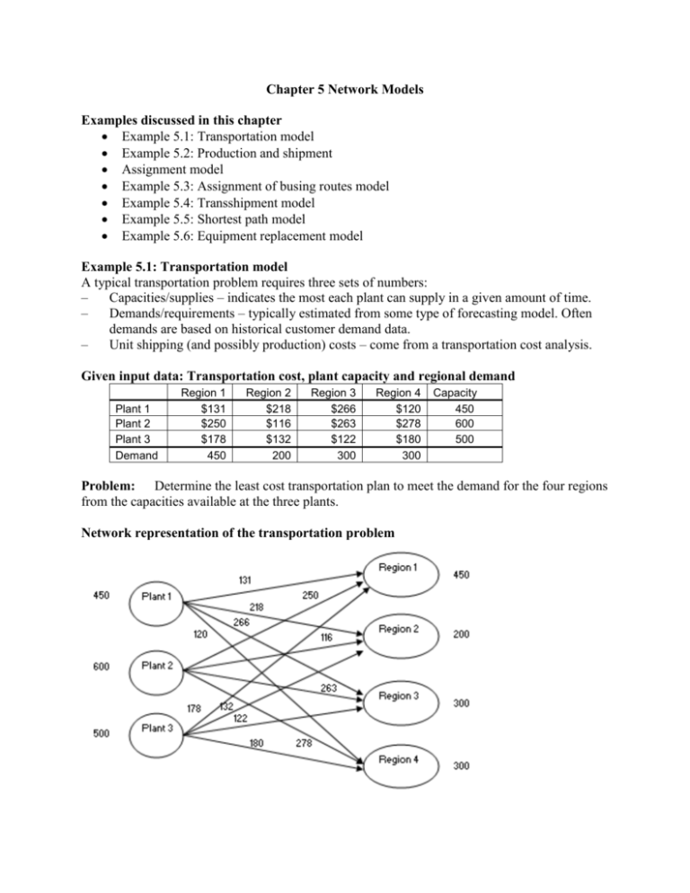
Network representation of the transportation problem
Decision variables: No. of automobiles sent from each plant to each region
Objective function: Minimize cost of transportation
Constraints:
Quantity shipped from a plan cannot exceed capacity
Quantity shipped to a region must meet its demand
Alternative Form of Transportation Model
Setup data as columns and use SUMIF function.
Example 5.2: Transportation model approach for maximizing profit when selling price and
cost of production are given.
Given input data
Table of transportation cost, plant capacity and regional demand as earlier
Selling price at the four regions
Cost of production at the three plants
Tax rate for profit generated at each plant
Problem: Develop a production and transportation plan that maximizes after-tax profit
Decision variables: No. of automobiles sent from each plant to each region
Constraints:
Quantity shipped from a plan cannot exceed capacity
Quantity shipped to a region must meet its demand
Objective function: Maximize after-tax profit
Profit per unit = (Selling price – Production cost – Shipping cost) * (1 – Tax rate)
§ 5.3 Assignment model
Assignment models are used to assign members of one set to members of another set in a least
cost or maximum profit manner. For example, suppose there are 4 jobs are 5 machines. Every
pairing of machine and a job has a given job completion time as below.
Machine
1
2
3
4
5
Job 1
14
2
7
2
5
Job 2
5
12
8
4
5
Job 3
8
6
3
6
4
Job 4
7
5
9
10
8
The problem is to find an assignment of machines to jobs such that the total completion time is
minimized.
Decision variables: Assignment of each machine to each job, 0 = not assigned, 1 = assigned
Objective function: Minimize cost completion time
Constraints:
Only one machine is assigned to a given job
No. of jobs assigned to a given machine does not exceed its capacity
Example 5.3 Assigning busing routes
Some assignments are not allowed, as in Bus Routing example.
Example 3: Minimum cost network flow model
Network flow models are like transportation models except:
 Capacity limits for transportation segments (arcs)
 Each node has inflows and outflows
 Shipment can be bi-directional
 Nodes are classified as “supplier”, “demanders”, and “transshipment points”
 “Supplier” nodes have capacity available
 “Demander” nodes have demand quantity required
 “Transshipment point” nodes have no supply and no demand
Graphical representation of problem 5.4 (Page 206)
Shipment costs are given in Table 5.7, page 206.
Input variables:
Decision variables:
Objective function:
Constraints:
Plant capacity, customer demand, arc capacity, shipment cost
Shipment on allowed arcs
Minimize total shipment cost
Flow on each arc <= capacity
Inflow and outflow must be balanced for each node as follows
Supply node: Outflow – Inflow <= available capacity
Demand node: Inflow – Outflow >= demand
Transshipment nodes: Inflow – outflow = 0
Optimal solution in network:
Sensitivity: Counting number of flows at capacity (Use COUNTIF)
Extensions:
 Two products on the flow network
 Perishable product, i.e. shrinkage in warehouse
Case 1: Two products on the flow network
Changes to the model:
 Two columns for arc flow, one for each product
 Arc capacity applies to the total flow of two products for each arc
 Set up two separate sets of flow balance constraints for each of the two products
Case 2: Product shrinkage in warehouses
Changes to the model:
 Assume a certain percentage of the product will be lost in the warehouse. In other words,
only a certain percentage of inflows go out as outflows. For example, if the shrinkage
factor is 90%, only 90% of the inflows will go out as outflows from warehouses; 10%
will be lost in warehouses.
 Then, the only the warehouse constraints need to be changed as follows:
Outflows – Shrinkage factor (Inflows) = 0
Example 4: Shortest path model
The problem is to find the shortest path between two points in a network. For example,
what is the shortest path between node 1 and node 10 in the network given in Figure 5.25 in page
214? The distance between each pair of nodes (arc) is given in the network.
This problem is similar to the Minimum cost network flow model discussed earlier, except,
 Node 1 is the “Supplier” node with a capacity of 1
 Node 10 is the “demander” node with a demand 1
 All other nodes are similar to warehouses where inflows must equal outflows
Extension: Equipment Replacement Model






Horizon is 5 years, i.e. 20 quarters
Purchase cost of a new machine is $3530 throughout the 5 years
Maintenance cost is $100 for first quarter, and increases by $65 per quarter for three
years
Salvage value of a machine is $1530 after the first quarter and decreases by $110/quarter
No machine is sold before the end of the first year
Machines remaining unsold at the end of three years are sold off
Objective: Optimal machine replacement strategy for five years
Shortest Path model for machine replacement problem
Nodes: Represent start of each quarter as a node. For a five year horizon we will have 21 nodes,
starting from node 1 representing the start of quarter 1 and node 21 representing the end
of quarter 20 (i.e. end of the fifth year).
Arcs: An arc between node “i” and node “j” represents purchase of a new machine at the
beginning of quarter “i” and selling it off at the beginning of quarter “j”. No arc is
required for the first 3 quarters of the life of the machine as machine are not sold within a
year. Also, no arcs are required past three years as machine not sold till three years are
sold off at the end of three years.
Arc (4,12) = Use the machine from quarter 4 to 11, and at the end of quarter 11 trade it in
for a new machine
Cost of an arc: Cost of arc = Maintenance cost for the duration of the arc – salvage value + Cost
of new machine
Cost of arc (4,12) = Maintenance cost for the first 8 quarters of the life of the machine Salvage value at the end of 8 quarter + Purchase price of a new machine
i.e. = (100 + 165 + 230 + 295 + 360 + 425 + 490 + 555) - (1530 – 7*110) + 3530 = $5390
Example 5: Project Scheduling
A project is defined by (i) a list of activities to be completed, (ii) duration of activity time for each
activity, and (iii) a list of immediate predecessors for each activity.
Activity (Node) Immediate predecessorsImmediate successorsDuration (weeks)
A
None
D, E
7
B
None
C
10
C
B
E
3
D
A
None
12
E
A, C
None
6
Forward scheduling
Earliest start time of a given activity (ES) = Max{Earliest finish time all its predecessors}
Earliest finish time of a given activity (EF) = ES + Duration
Backward scheduling
Latest finish time of a given activity (LF) = Min{Latest start time all its successors}
Latest start time of a given activity (LS) = LF - Duration
Slack of a given activity = LS – ES = LF – EF
An activity with zero slack is a critical activity. A path from start to finish using only critical
activities is called a critical path.
Example 5.7 Building a new room (Page 225)
Crashing the activities
Crashing an activity means reducing the activity time. Given cost of reducing activity time per unit
and a maximum limit for reduction, the task is to determine the least cost crashing to achieve the
desired project completion time.