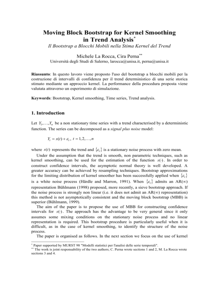
Moving Block Bootstrap for Kernel Smoothing
in Trend Analysis*
Il Bootstrap a Blocchi Mobili nella Stima Kernel del Trend
Michele La Rocca, Cira Perna**
Università degli Studi di Salerno, larocca@unisa.it, perna@unisa.it
Riassunto: In questo lavoro viene proposto l'uso del bootstrap a blocchi mobili per la
costruzione di intervalli di confidenza per il trend deterministico di una serie storica
stimato mediante un approccio kernel. La performance della procedura proposta viene
valutata attraverso un esperimento di simulazione.
Keywords: Bootstrap, Kernel smoothing, Time series, Trend analysis.
1. Introduction
Let Y1,, Yn be a non stationary time series with a trend characterised by a deterministic
function. The series can be decomposed as a signal plus noise model:
Yt  s(t )   t , t  1, 2,, n
where s (t ) represents the trend and  t  is a stationary noise process with zero mean.
Under the assumption that the trend is smooth, non parametric techniques, such as
kernel smoothing, can be used for the estimation of the function s () . In order to
construct confidence intervals, the asymptotic normal theory is well developed. A
greater accuracy can be achieved by resampling techniques. Bootstrap approximations
for the limiting distribution of kernel smoother has been successfully applied when  t 
is a white noise process (Härdle and Marron, 1991). When  t  admits an AR()
representation Bühlmann (1998) proposed, more recently, a sieve bootstrap approach. If
the noise process is strongly non linear (i.e. it does not admit an AR() representation)
this method is not asymptotically consistent and the moving block bootstrap (MBB) is
superior (Bühlmann, 1999).
The aim of the paper is to propose the use of MBB for constructing confidence
intervals for s () . The approach has the advantage to be very general since it only
assumes some mixing conditions on the stationary noise process and no linear
representation is required. This bootstrap procedure is particularly useful when it is
difficult, as in the case of kernel smoothing, to identify the structure of the noise
process.
The paper is organised as follows. In the next section we focus on the use of kernel
*
Paper supported by MURST 98 "Modelli statistici per l'analisi delle serie temporali".
The work is joint responsability of the two authors; C. Perna wrote sections 1 and 2, M. La Rocca wrote
sections 3 and 4.
**
smoothers for trend estimate and report some asymptotic results. In section 3 we
describe and discuss the MBB technique in trend analysis for the construction of
pointwise confidence intervals. Finally, in section 4 we report some results of a
simulation study where we compare the MBB with the asymptotic normal theory.
2. Kernel smoothers for trend analysis
Let s(t )  m0 (t / n) where m0  is a real smooth function on [0, 1]. We consider the
Nadaraya-Watson kernel smoother defined as:
n
 x t/n
1
ˆ
m( x)  m x, h, Y   (nh)  K 
Yt
h 
t 1 
The kernel function K  is a symmetric probability density and the bandwidth h is such


that h  O n 1 / 5 . Under some regularity conditions (Robinson, 1983) it is:
d
ˆ ( x)  m0 ( x)) 
(nh)1 / 2 (m

N (  ( x), 2 )
where:  ( x)  lim n (nh)1 / 2 bx and  2   2  K 2 x  dx with  2 being the variance
of the noise process and b( x )  h 2 m' ' ( x )  x 2 K x  dx . An approximate confidence
interval, of nominal level 1   , based on this limiting normal distribution is
mˆ x   ˆ n x  z / 2 where z is the quantile of order  of the standard normal
ˆ x. A bias corrected confidence interval
distribution and ̂ n2 x  is an estimate of Varm
ˆ x   bˆx   ˆ x  z
is given by m
where b̂ x  is an estimate of the bias b x  .
n
 /2
An alternative approach can be based on bootstrap schemes. They offer the advantage
of higher order accuracy with respect to the asymptotic normal approximations and they
are also able to correct for bias for kernel smoothers (Härdle and Marron, 1991). Here
we propose to use the MBB scheme for its wider range of applications. It gives
consistent procedures under some very general and minimal conditions. Moreover, this
is a genuine non parametric bootstrap method which seems the best choice when dealing
with nonparametric estimates. In our context, no specific and explicit structure for the
noise should be assumed. This can be particularly useful in kernel setting where the
specification of a smoothing parameter can heavily affect the structure of the residuals.
3. The moving block bootstrap procedure
Let Y  Y1 , Yn  be the observed time series. The bootstrap procedure runs as follows.
~
~
s t   m t / n, h , Y
Step 1. Fix a pilot bandwidth h and compute the estimates ~
for
t   n  1,, 1    n with 0    0.5 . Here the kernel smoother is used only in a


~
region  , 1    to avoid edge effects typical of kernel estimators. A pilot bandwidth h
is necessary for a successful approximation of the limiting distribution of m̂x  which
requires estimates of the asymptotic bias as well. Explicit estimates of this quantity can
be avoided by over-smoothing, that is by choosing a pilot bandwidth of larger order than
~
n 1/ 5 , i.e. h n1/ 5   .
Step 2. Compute the residuals ~t  Yt  ~
s t  with t  n   n  1, , 1    n.
Step 3. Fix l  card n  and form blocks of length l of consecutive observations
, i  1, 2,, 1   n. Let B*, B*,, B* be iid from
B  ~
,  , ~
i
 n i
 n i l 1
1
2
p
B1 , B2 ,, B1 n and construct the bootstrap replicate  *n1,,  *1 n. Generate
the bootstrap observations by setting. Yt*  ~
s t    t* with t  n . If card n  is a
multiple of l then p  card n / l , otherwise p  card n / l   1 and only a portion
of the p-th block is used.
~
Step 4. Compute m *  x   m x, h , Y * .
ˆ x   m0 x  with the bootstrap distribution of
Step 5. Approximate the distribution of m
~  x  , where m
~  x   m x, h~, Y .
m* x   m
As usual the bootstrap distribution can be approximated through a Monte Carlo
approach by repeating B times the steps 3-4. The empirical distribution function of these
B replicates can be used to approximate the bootstrap distribution of m̂x  .
ˆ x   m0 x  an approximate bootstrap confidence
Based on the non pivotal quantity m
interval of nominal level 1   is given by mˆ x   cˆ1 / 2 , mˆ x   cˆ / 2  where ĉ is the
quantile of order  of the bootstrap distribution.




4. Monte Carlo results and some concluding remarks
To study the characteristics of the proposed moving block procedure in terms of
coverage probabilities and to compare it with the classical asymptotic normal
approximations a small Monte Carlo experiment was performed. We considered the
same trend model m0 x  2  5x  5 exp( 100( x  0.5)2 ) , with x  0, 1 as in
Bühlmann (1998). As noise structures we used an ARMA(1,1) and an EXPAR(2) with
iid innovations distributed as a Student-t with 6 degrees of freedom, scaled so that
Var t   1 . All the simulations are based on 1000 Monte Carlo runs and 999 bootstrap
replicates. We fixed n  140 and 1    0.90 . The probability coverage is measured at
x  1 / 2 , the peak of the trend function. We considered a Normal kernel function with
~
smoothing parameters, h and h , varying according to Table 1.
In all the cases, bootstrap outperforms normal based procedures and in most cases it
outperforms normal based procedure with bias correction as well (see Table 2). The
specification of the smoothing parameter is crucial both for the bootstrap based
confidence intervals and the normal based ones, although the bootstrap method seems to
be overall less sensitive to it. Moreover a proper choice of the smoothing parameter
seems to be more important than that of the block length in the moving block procedure.
~
Our numerical results confirm that the pilot bandwidth h used in the MBB should be
larger than h.
~
~
Table 1. Bandwidth configurations. h  k1 0.044n 1 / 5 and h  h or h  k2 h5 / 9 .
h
~
h
C1
C2
C3
C4
C5
C6
C7
C8
C9
C10 C11 C12
.016
.016
.016
.051
.016
.102
.016
.204
.033
.033
.033
.075
.033
.150
.033
.300
.066
.066
.066
.110
.066
.220
.066
.440
Table 2. Pointwise empirical coverage at x=0.5. Noise model: ARMA(1,1) and
EXPAR(2) with residual distributed as T6. N: normal based confidence interval; NBC:
bias corrected normal based confidence interval; BT: MBB confidence interval.
ARMA
N
NBC
BT
EXPAR
N
NBC
BT
l
2
4
6
8
10
12
l
2
4
6
8
10
12
C1
.313
.140
.458
.411
.406
.296
.404
.398
C2
.316
.670
.719
.723
.804
.728
.731
C3
.310
.850
.913
.924
.948
.923
.925
C4
.307
.951
.975
.977
.988
.973
.977
C5
.453
.385
.461
.455
.450
.449
.444
.443
C6
.500
.607
.703
.728
.750
.739
.745
C7
.512
.751
.829
.866
.886
.891
.886
C8
.470
.830
.937
.963
.968
.965
.970
C9
.082
.568
.160
.198
.222
.239
.251
.250
C10
.582
.086
.144
.192
.213
.242
.259
C11
.284
.089
.194
.297
.358
.417
.449
C12
.115
.068
.217
.377
.497
.596
.672
C1
.174
.155
.337
.277
.267
.181
.266
.270
C2
.153
.633
.697
.704
.779
.706
.704
C3
.177
.852
.931
.931
.959
.930
.937
C4
.172
.954
.989
.991
.997
.990
.987
C5
.508
.278
.468
.461
.448
.426
.425
.430
C6
.424
.666
.730
.748
.757
.757
.755
C7
.495
.756
.824
.857
.882
.879
.883
C8
.516
.805
.898
.948
.966
.965
.966
C9
.164
.451
.313
.357
.372
.379
.382
.379
C10
.614
.195
.274
.334
.366
.386
.395
C11
.393
.180
.320
.424
.480
.512
.535
C12
.208
.145
.324
.464
.550
.619
.649
References
Bühlmann P. (1998) Sieve Bootstrap for Smoothing in Nonstationary Time Series, The
Annals of Statistics, 26, 48-83.
Bühlmann P. (1999) Bootstrap for Time Series, Research report n. 87, ETH, Zürich.
Robinson P.M. (1983) Nonparametric Estimation for Time Series Analysis, Journal of
Time Series Analysis, 4, 185-207.
Härdle, W., Marron, J. S. (1991) Bootstrap Simultaneous Error Bars for Nonparametric
Regression, The Annals of Statistics 19, 778-796.