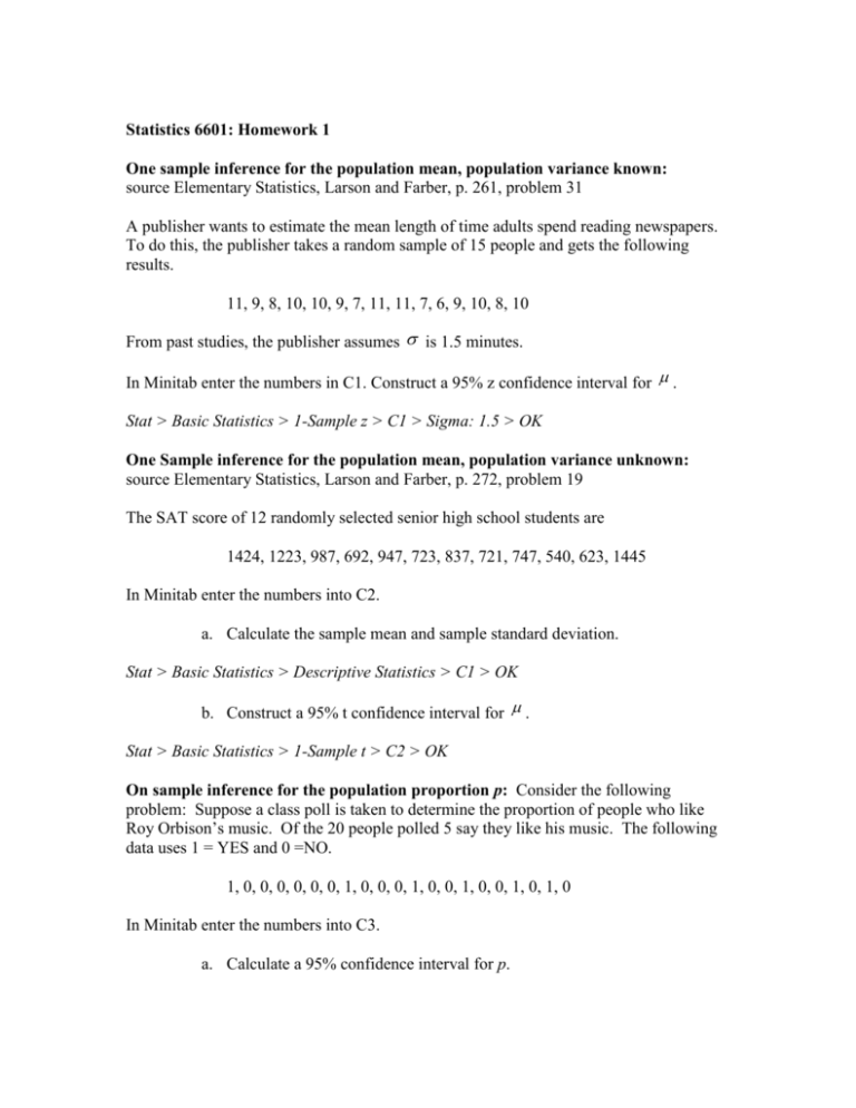
Statistics 6601: Homework 1
One sample inference for the population mean, population variance known:
source Elementary Statistics, Larson and Farber, p. 261, problem 31
A publisher wants to estimate the mean length of time adults spend reading newspapers.
To do this, the publisher takes a random sample of 15 people and gets the following
results.
11, 9, 8, 10, 10, 9, 7, 11, 11, 7, 6, 9, 10, 8, 10
From past studies, the publisher assumes  is 1.5 minutes.
In Minitab enter the numbers in C1. Construct a 95% z confidence interval for  .
Stat > Basic Statistics > 1-Sample z > C1 > Sigma: 1.5 > OK
One Sample inference for the population mean, population variance unknown:
source Elementary Statistics, Larson and Farber, p. 272, problem 19
The SAT score of 12 randomly selected senior high school students are
1424, 1223, 987, 692, 947, 723, 837, 721, 747, 540, 623, 1445
In Minitab enter the numbers into C2.
a. Calculate the sample mean and sample standard deviation.
Stat > Basic Statistics > Descriptive Statistics > C1 > OK
b. Construct a 95% t confidence interval for  .
Stat > Basic Statistics > 1-Sample t > C2 > OK
On sample inference for the population proportion p: Consider the following
problem: Suppose a class poll is taken to determine the proportion of people who like
Roy Orbison’s music. Of the 20 people polled 5 say they like his music. The following
data uses 1 = YES and 0 =NO.
1, 0, 0, 0, 0, 0, 0, 1, 0, 0, 0, 1, 0, 0, 1, 0, 0, 1, 0, 1, 0
In Minitab enter the numbers into C3.
a. Calculate a 95% confidence interval for p.
Stat > Basic Statistics > 1 Proportion > C3 > OK
One-way ANOVA Example: source Ott
Suppose a horticulturist was investigating the phosphorus content of tree leaves from
three different varieties of apple trees (1, 2, and 3). Random samples of five leaves from
each of the three varieties were analyzed for phosphorus content. The data are given
below. Use these data to test the hypothesis of equality of the mean phosphorus levels for
the three varieties. Use  = 0.05.
Row Variety1 Variety2 Variety3
---------------------------------1
0.35
0.65
0.60
2
0.40
0.70
0.80
3
0.58
0.90
0.75
4
0.50
0.84
0.73
5
0.47
0.79
0.66
--------------------------------------------------In SAS use Solution > Analysis > Analyst to produce the statistical analysis. Enter in
column A the Variety and in column B the phosphorus content.
Graphs > Boxplot, B Analysis, A Class
gives a boxplots
Statistics > ANOVA > One-Way ANVA, B Dependent, A Indepenent, Tests, Barletts’s
Test, Levene’s Test
Statistics > ANOVA > Nonparametric One-Way ANOVA, Test Calculate Exact p-values
Regression Example: source Applied Linear Regression Models, 3rd Edition, Neter,
et.al., p. 39, problem 1.21
Airfreight breakage. A substance used in biological and medical research is shipped by
airfreight to uses in cartons of 1,000 ampules. The data below, involving 10 shipments,
were collected on the number of times the carton was transferred from one aircraft to
another overt the shipment route (X) and the number of ampules found to be broken upon
arrival (Y). Assume that first-order regression model is appropriate.
Y
X
----------16.0 1.0
9.0 0.0
17.0 2.0
12.0 0.0
22.0 3.0
13.0 1.0
8.0 0.0
15.0 1.0
19.0 2.0
11.0 0.0
-----------In SAS use Solution > Analysis > Interactive Data Analysis to produce the statistical
analysis. Open in the WORK library.
Analyze > Scatter Plot (X,Y)
Analyze > Distribution Y
Analyze > Distribution (X,Y)
Analyze > Fit (X,Y)
gives a scatter plot
gives univariate statistics
gives bivariate statistics
give regression analysis
Write down the estimated regression model and test whether the slope of the line is zero.
Give a 95% CI for the slope.
Or use SAS use Solution > Analysis > Analyst to produce the statistical analysis.
Bootstrap:
The SAT score of 12 randomly selected senior high school students are
1424, 1223, 987, 692, 947, 723, 837, 721, 747, 540, 623, 1445
Bootstrap the mean using Resampling Procedures.
Use the editor in the software to create the file sas.dat. File > New Type in the following
data lines. The first line is the sample size. File > Save as sat.dat Done
12
1424
1223
987
692
947
723
837
721
747
540
623
1445
Perform the Bootstrap analysis of the mean using Analysis > Bootstrap Procedures >
Bootstrapped Mean First open the data File > Open sat.dat After loading the data click
Run
Fill in the following table by running the program 5 times. What do you notice about the
Bootstrap distribution as the number of repetitions increases? How do the Bootstrap
results compare to your previous results using the t-distribution?
NReps
Obtained
Mean
Lower
CI
Upper
CI
St.Error of
Bootstrap
Distibution
1,000
2,000
5,000
10,0000
50,000
Randomization Testing: source An Introduction to the Bootstrap, Efron and Tibshirani,
page 11
Sixteen mice were randomly assigned to a treatment group (n1 = 7) or a control group (n2
= 9). Shown are their survival times, in days, following a test surgery. Did the treatment
prolong survival?
Treatment 94 197 16 38 99 141 23
Control 52 104 146 10 50 31 40 27 47
Run the 2 independent samples randomization test using Resampling Procedures.
Use the editor in the software to create the file mouse.dat. File > New Type in the
following data lines. The first line is the sample sizes. File > Save as mouse.dat Done
79
94
197
16
38
99
141
23
52
104
146
10
50
31
40
27 47
Run the test Analysis > Randomization Tests > Two Independent Samples
First open the data File > Open mouse.dat After loading the data click Run
Fill in the following table by running the program 5 times. What do you notice about the
randomization distribution of the test statistics t? How do the randomization test results
compare with a standard two sample t-test using the t-distribution?
NReps
Obtained
t
% < -t,
% > +t
p more
extreme
effect
size
1,000
2,000
5,000
10,0000
50,000
If you have time try the analysis in StatXact. Enter Case Data > New
94
197
16
38
99
141
23
52
104
146
10
50
31
40
27
47
1
1
1
1
1
1
1
0
0
0
0
0
0
0
0
0
The run Statistics > Inference for Continuous Data > Two Independent Samples >
Premutation…