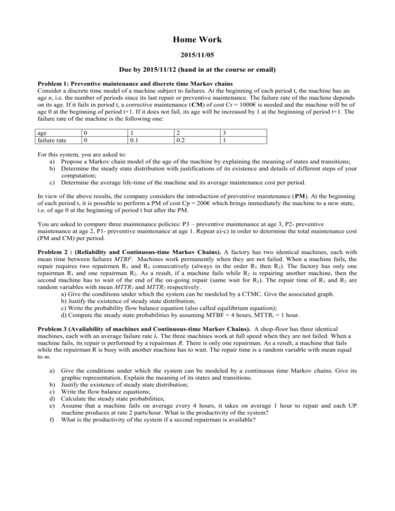
Home Work
2015/11/05
Due by 2015/11/12 (hand in at the course or email)
Problem 1: Preventive maintenance and discrete time Markov chains
Consider a discrete time model of a machine subject to failures. At the beginning of each period t, the machine has an
age n, i.e. the number of periods since its last repair or preventive maintenance. The failure rate of the machine depends
on its age. If it fails in period t, a corrective maintenance (CM) of cost Cr = 1000€ is needed and the machine will be of
age 0 at the beginning of period t+1. If it does not fail, its age will be increased by 1 at the beginning of period t+1. The
failure rate of the machine is the following one:
age
failure rate
0
0
1
0.1
2
0.2
3
1
For this system, you are asked to:
a) Propose a Markov chain model of the age of the machine by explaining the meaning of states and transitions;
b) Determine the steady state distribution with justifications of its existence and details of different steps of your
computation;
c) Determine the average life-time of the machine and its average maintenance cost per period.
In view of the above results, the company considers the introduction of preventive maintenance (PM). At the beginning
of each period t, it is possible to perform a PM of cost Cp = 200€ which brings immediately the machine to a new state,
i.e. of age 0 at the beginning of period t but after the PM.
You are asked to compare three maintenance policies: P3 – preventive maintenance at age 3, P2- preventive
maintenance at age 2, P1- preventive maintenance at age 1. Repeat a)-c) in order to determine the total maintenance cost
(PM and CM) per period.
Problem 2 : (Reliability and Continuous-time Markov Chains). A factory has two identical machines, each with
mean time between failures MTBF. Machines work permanently when they are not failed. When a machine fails, the
repair requires two repairmen R1 and R2 consecutively (always in the order R1 then R2). The factory has only one
repairman R1 and one repairman R2. As a result, if a machine fails while R2 is repairing another machine, then the
second machine has to wait of the end of the on-going repair (same wait for R2). The repair time of R1 and R2 are
random variables with mean MTTR1 and MTTR2 respectively .
a) Give the conditions under which the system can be modeled by a CTMC. Give the associated graph.
b) Justify the existence of steady state distribution;
c) Write the probability flow balance equation (also called equilibrium equation);
d) Compute the steady state probabilities by assuming MTBF = 4 hours, MTTRi = 1 hour.
Problem 3 (Availability of machines and Continuous-time Markov Chains). A shop-floor has three identical
machines, each with an average failure rate λ. The three machines work at full speed when they are not failed. When a
machine fails, its repair is performed by a repairman R. There is only one repairman. As a result, a machine that fails
while the repairman R is busy with another machine has to wait. The repair time is a random variable with mean equal
to m.
a) Give the conditions under which the system can be modeled by a continuous time Markov chains. Give its
graphic representation. Explain the meaning of its states and transitions.
b) Justify the existence of steady state distribution;
c) Write the flow balance equations;
d) Calculate the steady state probabilities;
e) Assume that a machine fails on average every 4 hours, it takes on average 1 hour to repair and each UP
machine produces at rate 2 parts/hour. What is the productivity of the system?
f) What is the productivity of the system if a second repairman is available?
Optional: (Packet switching and Continuous-time Markov Chains).
Consider a packet switching networking communication system composed of 3 nodes and 2 links:
The arrival process to node 1 is supposed to be Poisson with rate . All packets are transmitted through links 1-2 and 23. When node 3 receives a packet, it handles instantaneously the packet. All nodes have a limited capacity of one
packet. It implies:
- when a packet arrives at node 1 while node 1 is busy with another packet, the new packet is lost;
- if there is a packet on node 1 and another packet on node 2, then node 1 cannot start its emission till node 2 becomes
empty. It is assumed that node 1 is informed in real time of the availability of node 2.
The emission time of node i is assumed to be exponentially distributed with rate μi, i = 1, 2. The propagation on each
link is small enough to be neglected. While a packet is emitted, it occupies a place on the node.
a) Model the behavior of this network as a CTMC by indicating the meaning of each state;
b) Determine the stationary probabilities after the justification of their existence.
c) What is the probability of loss of a packet upon its arrival?
d) Give the average time a packet takes to traverse the network.
Problem 4. (Performance evaluation of Kanban-controlled system and stochastic Petri nets)
(You can use Excel solver to solve linear systems)
Consider a production system controlled by kanbans and illustrated by the figure below. It is composesd of two
machines M1 and M2. N kanbans are used to control the production. When there is at least one free kanban and there is
a part waiting in the input buffer of the system, a kanban is attached to the part and the part moves to the input buffer S1
of machine M1. After being served by M1, the part moves to the input buffer S2 of M2. After the service of M2, the
part waits in the finished good inventory S3 for a customer order. It is delivered when a customer order arrives. When
this happens, the kanban attached to the part is detached and sent to the free kanban buffer S4 and will be used to
authorize the production of other parts. Note that there are at most N parts in the system and the production is pulled by
customer demand.
demand
S4
S1
M1
S2
S5
M2
S3
lost
demand
Delivery
Input
Stock
free kanbans
Product flow
Part + Kanban
Demand flow
Part
Kanban flow
Fig. : A kanban-controlled system
In this problem, we assume that there is always a part in the input stock of the system. The processing times at M1 and
M2 are randomly variables of exponential distribution with mean 1/1 and 1/2. Customer demands arrive according to
a Poisson process at rate 0, i.e. the inter-arrival time is a random variable of exponential distribution of mean 1/0. A
customer demand is lost if the finished good inventory S3 is empty at its arrival. Let 0 = 1, 1 = 1.5, 2 = 1.5, .
S3 contains initially 2 parts and S1, S2, S4 and S5 are initially empty.
1. Model the system using stochastic Petri net. Be sure to explain the physical meaning of places and transitions. How
do you represent the lost demand?
2. Determine the structural properties of the model and explain their implications;
3. Determine the marking graph;
4.
5.
6.
7.
Determine the Markov chain;
Prove the existence of the stationary distribution;
Determine the stationary distribution of the Markov chain;
Determine the throughput rate, the percentage of lost demand, mean sojourn time of parts in S3.
Problem 5. (Dimensioning the number of beds : Target occupancy level and queueing network) Consider
obstetrics units in hospitals. Obstetrics is generally operated independently of other services, so its capacity needs can
be determined without regard to other services. It is also one for which the use of a standard M/M/s queueing model is
quite good. Most obstetrics patients are unscheduled and the assumption of Poisson arrivals has been shown to be a
good one in studies of unscheduled hospital admissions. In addition, the coefficient of variation (CV) of the length of
stay (LOS), which is defined as the ratio of the standard deviation to the mean, is typically very close to 1 satisfying the
service time assumption of the M/M/s model.
(Dimensioning the number of beds) Since obstetrics patients are considered emergent, the American College of
Obstetrics and Gynecology (ACOG) recommends that occupancy levels of obstetrics units not exceeding 75%. Many
hospitals have obsterics units operating below this level. However, some have eliminated beds to reduce « excess »
capacity and costs and 20% of NY hospitals had obstetrics units that would be considered over-utilized by this standard.
Assuming the target occupancy level of 75%, what is the probability of delay for lack of beds for a hospital with s = 10,
20, 40, 60, 80, 100, 150, 200 beds. (Excel is needed)
Lesson: For the same occupancy level, the probability of delay decreases with the size of the service.
Problem 6: Performance evaluation of a base-stock policy with backlogged demand
(Excel could be helpful)
M1
demand
M2
stock
production
Consider a system of two identical machines, each with a maximal production rate μ= 1 part/hour. A finished part is
immediately put in a stock. Customer demand arrives randomly at rate λ = 1.8 part/hour. A demand is satisfied
immediately if the stock is not empty. Otherwise, it is backlogged and waits for parts.
The following so-called base-stock policy is used to control the production: a machine finishing a part starts a new part
while the inventory position IP (equal to number of parts in stock – backordered demand+ number of parts being
processed by the machines) is below a so-called base-stock level S. When the base stock level S is reached, a machine
finishing a part is kept idle till the buffer level drops below S. Let X(t) be the stock level (number of parts in stock –
backordered demand) at time t.
a) (i) Show that X(t) is a CTMC (Continuous Time Markov Chains) under conditions that you will explain. (ii) Give
the graphic representation of the CTMC by giving the meaning of states and transitions;
b) Verify the conditions of the existence of steady state probabilities : irreducibility of the Markov chain and the
stability of the system;
c) Determine the steady state probabilities n;
d) Let S = 4. Determine the mean inventory level and the service ratio which is defined as the percentage of customer
demands satisfied immediately from stock;
e) Determine the base stock level S in order to achieve a service ratio of 95%;
f) How the mean inventory level and the service ratio change when S increases? Illustrate this relation by an
inventory-level vs service-ratio curve? How can one use this relation to correctly set base stock level?

Problem 7 (a tandem queueing network)
Consider a tandem production line composed of 3 workstations (M1, M2, M3). Each workstation is composed of a
machine and an upstream buffer. The maximal production rate is 1 = 5 parts/hour on M1, 2= 6 parts/hour on M2
and 3=5 parts/hour on M3. What are the average buffer level and the average production lead time for arrival rate =
3, 4, 4.5?
S1
M1
S2
M2
S3
M3