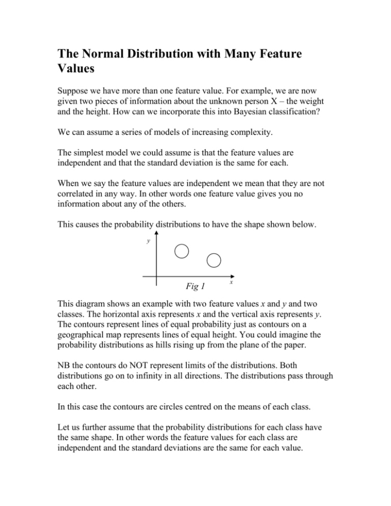
The Normal Distribution with Many Feature
Values
Suppose we have more than one feature value. For example, we are now
given two pieces of information about the unknown person X – the weight
and the height. How can we incorporate this into Bayesian classification?
We can assume a series of models of increasing complexity.
The simplest model we could assume is that the feature values are
independent and that the standard deviation is the same for each.
When we say the feature values are independent we mean that they are not
correlated in any way. In other words one feature value gives you no
information about any of the others.
This causes the probability distributions to have the shape shown below.
y
Fig 1
x
This diagram shows an example with two feature values x and y and two
classes. The horizontal axis represents x and the vertical axis represents y.
The contours represent lines of equal probability just as contours on a
geographical map represents lines of equal height. You could imagine the
probability distributions as hills rising up from the plane of the paper.
NB the contours do NOT represent limits of the distributions. Both
distributions go on to infinity in all directions. The distributions pass through
each other.
In this case the contours are circles centred on the means of each class.
Let us further assume that the probability distributions for each class have
the same shape. In other words the feature values for each class are
independent and the standard deviations are the same for each value.
Notice how the probability of belonging to a certain class depends on the
distance from the mean of that class. The distance d is given by
d 2  x2  y2
which is just Pythagoras theorem.
The decision boundary between two classes will be the set of points which
are equally distant from the means of both classes. This will be a straight
line which passes through the midpoint of the line joining the two means.
This line is known as the “perpendicular bisector” of the two means.
Now the next most complex model assumes that the feature values are still
independent but that the standard deviations are now different. This leads to
the situation shown below.
Fig 2
The probability contours are now elliptical and the axes of the ellipse are
parallel to the x and y axes.
Lets still assume that the shape of the probability distribution is the same for
each class. In other words only the position of the mean is different.
Now we can obtain Fig 1 from Fig 2 by a simple transformation. Imagine
that Fig 2 is drawn on a rubber sheet. If we squash the rubber sheet in the x
direction then we can convert the ellipses into circles. We could then draw a
decision boundary between the two classes. It will be the perpendicular
bisector between the two means.
We could then stretch the rubber sheet back to its original position. The
decision boundary will still be a straight line but its slope will have changed.
Alternatively we could also describe the probability distributions in terms of
distance from the means. But now we have to invent a new type of distance
metric
d2 
x2
 x2

y2
 y2
This is called Mahalanobis distance. The decision boundary is the set of
points with equal Mahalanobis distance from the two means.
The next most complex model assumes that the feature values are no longer
independent. Or, in other words, that they are correlated with one another.
This implies that if we know one feature value then this tells us something
about the other feature values.
The probability contours now look like this.
Fig 3
They are still elliptical but the axes of the ellipses are not parallel to the x an
y axis.
In the case shown here the principal axes slope upwards. This implies that as
x increases y also tends to increase. So if you know that x is high you would
expect y also to be high.
Let us still assume that the probability distributions have the same shape for
each class.
But we can turn Fig 3 into Fig 2 by a simple transformation. We simply
rotate the co-ordinate system so that the axes are now parallel to the axes of
the ellipse.
We can then squash the co-ordinate system to turn the ellipses into circles.
We can then draw the decision boundary as before. We can then stretch and
rotate the co-ordinate system back to its original state. The decision
boundary will still be a straight line.
The most complex model we can assume is that the feature values are not
independent and the probability distributions for the two classes have
different shapes.
One example of this is shown below.
Fig 4
The probability contours are still ellipses but the different classes are no
longer represented by the same ellipse.
Now the decision boundaries are no longer represented by straight lines. An
extreme example is shown below.
One class is represented by a broad shallow distribution but the other is
represented by a narrow highly peaked distribution. The second class is
concentrated in small region and is “surrounded” by the first class.
The decision boundary will be closed loop with a tail pointing away from the
mean of class 1.
In general the decision boundaries will be quadratic curves. These include
circles, ellipses, parabolas and hyperbolas.
The problem is that a quadratic curve requires many more parameters to
define it than a straight line.
If we have N feature values a line requires N parameters but a quadratic
curve requires N 2 .
In image analysis it is quite common to have images with more than 1000
pixels. Since each pixel counts as a feature value a quadratic curve would
require more than 1 million parameters.
To fit the values of 1 million parameters we would need over 1 million
objects in our training set. It is very rare that we have this amount of data.
For this reason, it is common practice to assume that all classes have the
same shape even when this is unlikely to be the case. If the classes have the
same shape then the decision boundaries are straight lines or planes and so
require far fewer parameters.
However, there is an alternative way of dealing with this problem. It is
called Principal Component Analysis.
Principal Component Analysis
The main purpose of Principal Component Analysis is to find the vectors
which represent the axes of the ellipsoids.
It turns out that these vectors are the eigenvectors of the covariance matrix.
The covariance matrix is defined as follows.
The covariance matrix is an NxN matrix where N is the number of feature
values. Lets suppose we have a set of objects each with N feature values.
The element  ij in the row i and column j represents the covariance of the ith
and jth feature values. Let the ith and jth feature values of the kth object be
called x k and y k then  ij is given by
 ij2   ( xk  m x )( y k  m y )
k
where m x is the mean of the ith feature value and m y is the mean of the jth
feature value.
Along the leading diagonal (where i=j)  ij is just the standard deviation of
the ith feature value. The off-diagonal elements are measures of how much
feature value i is correlated with feature value j. If  ij = 0 then i and j are
independent.
You can see from the above equation that  ij must equal  ji .This implies
that the covariance matrix is “symmetric”. That is if you were to flip the
matrix about the leading diagonal the matrix would remain unchanged. In
other words if you interchanged the rows and columns the matrix would
remain unchanged.
In the situations discussed above the covariance matrices are as follows.
When the probability contours are circles (Fig 1) the covariance matrix is
 2 0 


 0 2


The off-diagonal elements are zero because the feature values are
independent. The elements on the leading diagonal are all equal because the
standard deviation is the same for each feature value.
In the second situation where the probability contours were ellipses with
their axes parallel to the x and y axes (Fig 2) the covariance matrix is
  x2

 0

0 

 y2 
The off-diagonal elements are still zero because the feature values are still
independent. But the elements on the leading diagonal are no longer equal
because the standard deviations are different for each feature value.
In the third case where the probability contours were ellipses with their axes
at an angle (Fig 3) the covariance matrix is
  x2
 2

 xy
 xy2 

 y2 
The off-diagonal elements are no longer zero because the feature values are
no longer independent.
In the final most complex case which we considered above the classes had
probability distributions with different shapes (Fig 4). The covariance matrix
is a description of the shape of the probability distribution. In this case each
class would have a different covariance matrix.
Eigenvalues and Eigenvectors
The eigenvalues and eigenvectors of a square matrix A are defined by
Au k  k u k
where u k is the kth eigenvector and  k is the kth eigenvalue. If A is an NxN
matrix then there will be N eigenvectors and N eigenvalues. Each vector
u k will have N components. The eigenvalues  k are scalars.
(Here we use the convention that vectors are symbolised by lower-case bold
characters e.g. u, matrices by upper-case bold e.g. A and scalars by italic
e.g. s.)
The above equation says that if you multiply any eigenvector u k by the
matrix A you get the same eigenvector back again but multiplied by the
scalar  k .
We saw above that covariance matrices are symmetric. If A is symmetric
then the eigenvectors have the following two properties
 The eigenvectors form a “complete” set. This means that they can be
used as the axes of a co-ordinate system. Or, in other words, any Ndimensional vector can be expressed as a linear combination of the
eigenvectors.
 The eigenvectors are orthogonal
0 i  j
ui  u j  
1 i  j
Here u i  u j is the “dot” product or scalar product of the two vectors.
In addition the eigenvalues of a covariance matrix have another property.
They are all greater than or equal to zero
k  0
The eigenvectors of the covariance matrix represent the directions of the
principal axes of the ellipsoids. The eigenvalues represent the squares of the
standard deviations along those axes.
u2
u1
The eigenvectors are ranked in order of the size of their eigenvalues. So u1
is the eigenvector with the largest eigenvalue. u1 represents the axis along
which the ellipsoid is widest. 1 is proportional to the square of the width of
the ellipsoid along that axis.
u 2 is at right angles to u 1 and represents the axis along which the ellipsoid is
next widest.  2 is proportional to the square of the width of the ellipsoid
along that axis.
In N-dimensional space an ellipsoid will have N axes all at right angles to
one another. u k represents the kth axis and  k is proportional to the square
of the width of the ellipsoid along that axis.
We can now transform the co-ordinate system of feature space so that the
eigenvectors now define the axes. This means that the data is now described
by a new set of feature values. The new feature values are given by taking
the dot product of the old feature vector with each eigenvector in turn.
When the data is expressed in terms of the new feature values the axes of the
ellipsoids are now parallel to the axes of the co-ordinate system. So the
feature values are now independent of each other. The off-diagonal elements
of the new covariance matrix are zero. The new covariance matrix is
 12

0

0
 

0
0

2
2
0
0
32


0 

0 

0 
 
where the diagonal elements are the eigenvalues. Remember the eigenvalues
are equal to the square of the standard deviations along the axes.
It is usually the case that if N is large (say > 50) the eigenvalues fall very
steeply
k
k
This means that the data is spread out in only a small number of directions.
There are only a small number of axes of the ellipsoid where the ellipsoid is
significantly wide. Along all the other axes the ellipsoid is very thin.
You can visualise this by considering a 3-dimensional space, for instance a
room in a building, and imagining that the data is spread out on the surface
of a table within the room. The data is spread out along only two
dimensions. It has very little variation perpendicular to the surface of the
table. So the third dimension gives us very little information about the data.
We can now ignore all those feature values whose eigenvalues are below a
certain threshold. The data has very little variation along these directions.
The data is described almost completely by the small number of feature
values with large eigenvalues.
This means that we have reduced the number of dimensions N necessary to
describe the data. Typically we can reduce N from > 50 down to maybe 5 or
6. But remember that the number of parameters needed to describe a
quadratic curve is proportional to N 2 . So we reduce the number of
parameters from > 2500 down to 25 or 36. This is a huge reduction in the
complexity of the model.
This is the basic reason why we use Principal Component Analysis. It
reduces the number of dimensions and allows us to use simpler models.
What do the Principal Components mean?
The eigenvectors usually represent independent modes of variation in the
data. Often these represent underlying “causes” in the real world which lead
to the different manifestations of the data.
For example, consider the distribution of height and weight among the male
population
weight
B
C
A
D
height
Here the main axis of the ellipse slopes upward showing that height and
weight are correlated. The second axis is perpendicular to the main axis.
These two axes form a “natural” co-ordinate system to describe the data. But
what do these two axes represent in the real world?
Consider the people around points A and B at opposite ends of the main
axis. People at point A have low weight and low height so they are small
people but have a normal body shape. People at point B have high weight
and high height so they are large people but also have a normal body shape.
So the main axis represents a change in size of the person while the body
shape remains constant.
A
B
Consider people at points C and D at opposite ends of the secondary axis.
People at point C have low weight but high height so they are very thin
people. People at point D conversely have high weight and low height so
they are very fat people. So the secondary axis represents a change in body
shape from thin to fat. You could call this the “obesity” axis.
C
D
Lets take a more complicated example. Suppose we gathered many
thousands of hand-written examples of the digit ‘2’. We could find the
Principal Components of this data. We would probably find that some of the
eigenvectors represented variations like these:
A variation in the tilt of the main axis
A variation in the height of the upper loop
A variation in the size of the lower loop
A variation in the angle of the downstroke
Some Vector Mathematics
The easiest way to calculate decision boundaries is to use vector
mathematics.
b
c1
m
c2
In the simplest case where the distributions are circles it is very easy to
calculate the equation of the boundary. The boundary passes through the
midpoint m between the means of the two classes, where
m  (c1  c 2 ) / 2
Let the vector b represent the direction of the boundary. Let the vector n
represent the vector between the two means.
n  c 2  c1
The boundary b is perpendicular to n. Therefore
b.n  0
We have a choice as to the exact values of the components of b. There are a
number of possibilities that will satisfy the above equation but the simplest
choice is to make
b1  n2
b2  n1
Now we can represent the equation of the boundary by
p = m + sb
where p represents the position vector of any point on the boundary and s is
a scalar.
This also gives us an easy way of deciding which class a new object is in.
Let the feature values of the new object be vector d. Then if
(d-m).n >0
then it’s in class 1 and if it’s < 0 then it’s in class 2.
Now let’s see how to find the decision boundary in the case where the
probability distributions are elliptical. At the start of this chapter we said that
you could convert Fig 2 to Fig 1 by “squashing up” the axes so that the
ellipses became circles.
We can squash up the axes by dividing the x-values by  x and the y-values
by  y . This means that the standard deviations along both axes are now
equal to 1. The components of the vector n between the two means now
become
n1 /  x
n2 /  y
The vector b which represents the boundary now becomes
b1  n2 /  y
b2  n1 /  x
We now have to “unsquash” the axes in order to return to the original state.
So we now have to multiply the x-values by  x and the y-values by  y . The
components of the boundary vector now become
b1 
x
n2
y
b2  
y
n1
x
The decision boundary still passes through the midpoint between the two
means but the slope has now changed. So we can still write the equation of
the boundary as
p = m +sb
Its just that the values of b are different.
Now let us consider the third situation where the ellipses are at an angle. We
now have to rotate the x and y axes so that they are parallel to the axes of the
ellipse.
Let u1 and u 2 be the eigenvectors which represent the first and second axes
of the ellipses. Then if we rotate the x and y axes the new values of the
components of n become
n1  n.u1
n2  n.u 2
This gets us back to situation 2 so we now have to squash up the axes again
so that the ellipses become circles. So just as before we divide the
components of n by  1 and  2 , the standard deviations along the first and
second axes.
n1 /  1
n2 /  2
Of course,  1 is just  1 and  2 is  2 where 1 and  2 are the
eigenvalues. We can now set the values of b as before
b1  n2 /  2
b2  n1 /  1
Then we have to unsquash the axes
1
n2
2

b2   2 n1
1
b1 
And finally rotate them back to the original angles.
b1  b.v
b2  b.w
where v and w are the vectors in the rotated co-ordinate system which
represent the original x and y axes
v1  (1,0).u1
v2  (1,0).u 2
w1  (0,1).u1
w2  (0,1).u 2
Vectors and Principal Components
We saw above that Principal Components Analysis tells us which are the
most important eigenvectors. These eigenvectors are the directions in
feature space which best describe the data.
Take for example the graph below which shows the eigenvalues
k
All the eigenvalues except the first three are nearly zero. In other words only
the first three eigenvectors give any useful information about the data. The
variation in the data along the remaining eigenvectors is negligible. This
implies that the data lies in a three-dimensional sub-space within the total
feature space.
During the classification phase, when we wish to classify a new object, we
could simply test to see if the new object lies in the above three-dimensional
space. If it does not then we know that the object cannot belong to the class
represented by the above data. But how can we decide whether the new
object lies in this space?
Let us choose some point within the space to be the origin (the most
convenient point to choose would be the mean). Let the new object be
represented by point P. Then let us draw the vector from the origin to P.
Let’s call this vector p.
If P lies in the space then the scalar product of p with any of eigenvector u k
where k > 3 will be very small. We could calculate each of these values and
test to see if they are small but this is not very computationally efficient
since there may be many such eigenvectors.
It’s easier to use the following formula
N
3
 p g
i 1
2
i
k 1
2
k
T
which is equivalent to the above operation but is faster since it only involves
calculating three scalar products.
Here N is the total number of dimensions and
g k  p.u k
is the scalar product of p with eigenvector u k .
T is a threshold value which the user is free to choose. But usually T will
depend on the eigenvalues which are left out of the sub-space. So a
reasonable choice would be
N
T  3  j
j 3