1
CHAPTER 3
3.1 (a)
(101101) 2  (1  2 5 )  (0  2 4 )  (1  2 3 )  (1  2 2 )  (0  21 )  (1  2 0 )
 32  8  4  1  45
(b)
(101.101) 2  (1  2 2 )  (0  21 )  (1  2 0 )  (1  2 1 )  (0  2 2 )  (1  2 3 )
 4  1  0.5  0.125  5.625
(c)
(0.01101) 2  (0  2 1 )  (1 2 2 )  (1 2 3 )  (0  2 4 )  (1 2 5 )
 0.25  0.125  0.03125  0.40625
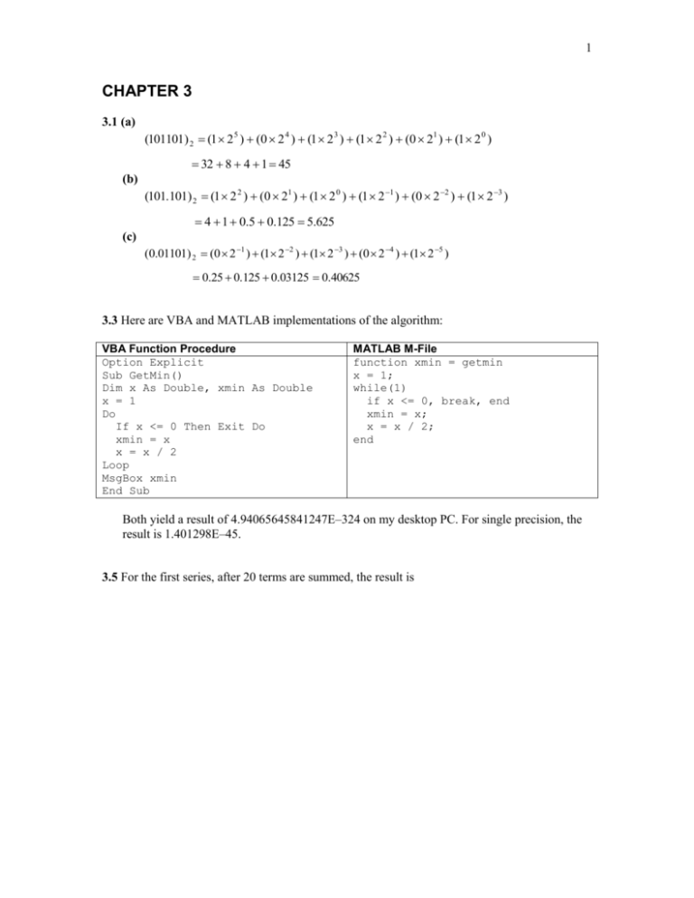
3.3 Here are VBA and MATLAB implementations of the algorithm:
VBA Function Procedure
Option Explicit
Sub GetMin()
Dim x As Double, xmin As Double
x = 1
Do
If x <= 0 Then Exit Do
xmin = x
x = x / 2
Loop
MsgBox xmin
End Sub
MATLAB M-File
function xmin = getmin
x = 1;
while(1)
if x <= 0, break, end
xmin = x;
x = x / 2;
end
Both yield a result of 4.94065645841247E–324 on my desktop PC. For single precision, the
result is 1.401298E–45.
3.5 For the first series, after 20 terms are summed, the result is
2
The result oscillates at first. By n = 20 (21 terms), it is starting to converge on the true value.
However, the relative error is still a substantial 0.11%. If carried out further to n = 27, the
series eventually converges to within 7 significant digits.
In contrast the second series converges much faster. It attains 6 significant digits by n = 20
with a percent relative error of 8.110–6%.
3
3.7 First, the correct result can be calculated as
y  1.37 3  7(1.37) 2  8(1.37)  0.35  0.043053
(a) Using 3-digits with chopping
1.373
–7(1.37)2
8(1.37)



2.571353
–7(1.87)
10.96



2.57
–13.0
10.9
– 0.35
0.12
This represents an error of
t 
0.043053  0.12
 178.7%
0.043053
(b) Using 3-digits with chopping
y  ((1.37  7)1.37  8)1.37  0.35
y  (5.63  1.37  8)1.37  0.35
y  (7.71  8)1.37  0.35
y  0.29  1.37  0.35
y  0.397  0.35
y  0.047
This represents an error of
t 
0.043053  0.047
 9.2%
0.043053
Hence, the second form is superior because it tends to minimize round-off error.
3.9 Here is a MATLAB M-file to solve the problem. Programs in other languages would have a
similar structure and outcome.
%
%
%
%
Given: Taylor Series Approximation for
cos(x) = 1 - x^2/2! + x^4/4! - ...
Find: number of terms needed to represent cos(x) to
8 significant figures at the point where: x = 0.3 pi
x = 0.3 * pi;
es = 0.5e-08;
4
%approximation
cosi = 1;
j = 1;
% j=terms counter
fprintf('j= %2.0f cos(x)= %0.10f\n', j,cosi)
fact = 1;
while(1)
j = j + 1;
i = 2 * j - 2;
fact = fact * i * (i - 1);
cosn = cosi + ((-1) ^ (j + 1)) * ((x) ^ i) / fact;
ea = abs((cosn - cosi) / cosn);
fprintf('j= %2.0f cos(x)= %0.10f ea = %0.1e\n',j,cosn,ea)
if ea < es, break, end
cosi = cosn;
end
j=
j=
j=
j=
j=
j=
j=
1
2
3
4
5
6
7
cos(x)=
cos(x)=
cos(x)=
cos(x)=
cos(x)=
cos(x)=
cos(x)=
1.0000000000
0.5558678020
0.5887433702
0.5877699636
0.5877854037
0.5877852513
0.5877852523
ea
ea
ea
ea
ea
ea
=
=
=
=
=
=
8.0e-001
5.6e-002
1.7e-003
2.6e-005
2.6e-007
1.7e-009
The true value of cos(0.3) is 0.5877852525. Therefore, 6 terms of the Maclaurin series are
necessary to approximate the true value to 8 significant figures.
3.11 Remember that the machine epsilon is related to the number of significant digits by Eq. 3.11
  b1t
which can be solved in base 10 for a machine epsilon of 1.19209107 for
t  1  log 10 ( )  1  log 10 (1.19209  10 -7 )  7.92
To be conservative, assume that 7 significant figures are good enough. Recall that Eq. 3.7 can
then be used to estimate a stopping criterion,
 s  (0.5  10 2n )%
Thus, for 7 significant digits, the result would be
 s  (0.5  10 27 )%  5  10 6 %
The total calculation can be expressed in one formula as
 s  (0.5 10 2Int(1log10 ( )) )%
5
It should be noted that iterating to the machine precision is often overkill. Consequently,
many applications use the old engineering rule of thumb that you should iterate to 3
significant digits or better.
As an application, I used Excel to evaluate the second series from Prob. 3.5. The results are:
Notice how after summing 21 terms, the result is correct to 7 significant figures. At this point,
the true and the approximate percent relative errors are at 1.82106% and 6.29106%,
respectively. The process would repeat one more time so that the error estimates would fall
below the precalculated stopping criterion of 5106 %.