Bipartie Matchings
PHAM Thuy Lien
1. Introduction
The bipartite matching problem is a problem of network optimization. It is possible to view
the models of this problem in the act, and one of the applications known is the assignment
problem. This problem is also a technique for resolve a model of the scheduling problem. This
document resolves this problem in two aspects: deterministic and randomized, with the
probability that has the error with the randomized algorithm for finding a perfect matching is
at most ½.
Keywords: assignment problem, perfect matching, randomized algorithm.
2. Matching problem
Let G=(V,E) be a undirected simple graph (no multiple edges), each of whose edges has a
real-valued weight, denoted by weight(v,w).
A matching M on G is a set of edges joining disjoint vertices, i.e. no two of which
have a common vertex:
+ The size |M| of M is the number of edges it contains.
+ The weight of M is the sum of its edge weights.
The maximum matching problem is that of finding a matching of maximum size or
weight. There are four versions of this problem, depending on whether we want to maximize
size or weight and whether G is bipartite or not.
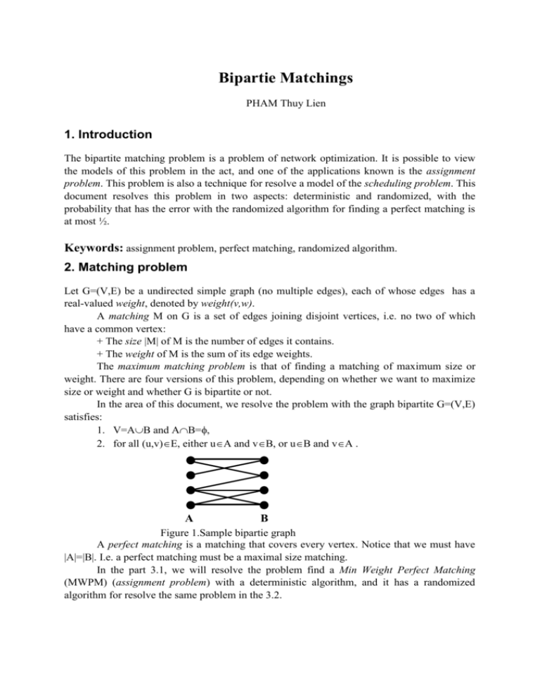
In the area of this document, we resolve the problem with the graph bipartite G=(V,E)
satisfies:
1. V=AB and AB=,
2. for all (u,v)E, either uA and vB, or uB and vA .
A
B
Figure 1.Sample bipartie graph
A perfect matching is a matching that covers every vertex. Notice that we must have
|A|=|B|. I.e. a perfect matching must be a maximal size matching.
In the part 3.1, we will resolve the problem find a Min Weight Perfect Matching
(MWPM) (assignment problem) with a deterministic algorithm, and it has a randomized
algorithm for resolve the same problem in the 3.2.
3. Descriptions and functions of the implemented solutions
3.1 The deterministic algorithm for the problem of MWPM
In this part, the algorithms work with the ganeral case, |E|=n x n (By adding the pseudo-edge
with enough grand weight).
3.1.1 The exhaustive algorithm
This algorithm realize to search all perfect matching possible and holds the best result.
Consequentially it can’t be applied when n is grand.
The basic recursive procedure for exhaustive enumeration base on the method of
backtracking search, is:
Procedure SearchPerm(i:integer, mark:array[1..n])
{for a permutation reached}
Begin
for y =1 to n do
if mark[y]=0 then
begin
perm[i] = y;
mark[y]=1;
if i=n then TestPerm(perm)
else SearchPerm(i+1);
mark[y] = 0;
end
end
Procedure TestPerm(perm)
{test a permutation if it is satisfied or not}
begin
if weight(M(perm))< Weight then
//update and hold new weight, new perm
end
Then we begin with the call from i=1:
Procedure Main
begin
For i=1 to n do mark[i]=0;
Weight = MAX; {A value enough grand}
SearchPerm(1);
end
3.1.2 The algorithm base on finding and breaking the negative cycle
Notion of algorithm base on the assignment labels to the edges. The edges of matching
have negative values and the rest have positive values. Begin with one possible matching, the
algorithm realizes the search of negative cycles in the graph, if found, breaks this cycle by
change the sign of edges, actually have changed the matching whose weight is smaller. This
process is continued until there doesn’t exist any negative cycle.
Example is shown in figure following:
-7
2
A
7
8
-5
-2
B
Figure 2. A negative cycle is found
(costcycle= -2)
A
-8
5
B
Figure 3.Change matching
The procedure of finding and breaking negative cycle bases on the Ford-Bellman
algorithm (O(n3)), in order to find a shortest path from a vertice to rest of one part of the
bipartite graph. Let da[] is label of set of vertex of A, db[] is label of set of vertex of B. From
the matrix of weight c[i][j], iA, jB, we compute the upper bound da[i] for vertice i of A to
vertice j of B, each time we detect:
da[i] > db[j] + c[i][j]
then the upper bound da[i] is better by :
da[i] = db[j] + c[i][j]
3.2 The randomized algorithm for the problem of MWPM
We describe the algorithm begin to decide whether there is a perfect matching in a
graph G bipartite, after find min weight one, if such exists.
3.2.1 Determining whether G has a perfect matching
Consider the adjacency matrix A on graph G whose entries aij are defined as follows:
(1) aij = 1 if (i,j)E
= 0 otherwise
where the indices i and j correspond to vertices of the vertex sets A and B respectively.
There exists a perfect matching in the graph G if and only if the adjacency matrix
contains a set of n 1’s, no two of which are in the same column or row. In other words, if all
other entries were 0 a permutation matrix would result.
Consider the function called the permanent of A, defined as follows:
(2) perm(A) =  (i=1n ai) where  is a permutation of set 1..n
This gives the number of perfect matchings of the graph A represents. Unfortunately the best
known algorithm for conputing the permanent has running time O(n2n). However, note the
similarity of the formula for computing the permanent to that for the determinant of A:
det(A) =  sign() (i=1n ai)
where sign() =1 if  is product of even number of transpositions and sign()=-1 otherwise.
The determinant can be computed in O(n3) time by using Gaussian elimination (and
in O(log2(n)) time on O(n3,5) processors). Note also that:
det(A)0  perm(A)0   perfect matching
Unfortunately the converse is not true.
To handle the converse, we replace each entry aij of matrix A with (aijxij), where xij is a
variable. Note both det(A’) and perm(A’) are polynomials in xij. It follows:
det(A)0  perm(A) 0  ! perfect matching
Then define matrix A’ as:
A= 0
if (i,j) E
(1)
= xi j if (i,j) E, i<j
= -xij if (i,j) E, i>j
The determinant of A’ is a poltnomial in n2 variables. We will see that this determinant is
different from 0 if and only if there is a perfect matching in G. To formulate an algorithm to
determine if there is a perfect matching, we base on the theorems follows:
Theorem 2.1 (Tutte) det(A)  0 iff A has a perfect matching
Theorem 2.2 (Rabin-Vazirani) Let the values of the xij be independently and uniformly
distributed in [1,2,..,2n], where n=|A|=|B|. Let A’ be the resulting matrix. Then
Pr[det(A’)=0 | det(A)! 0]  ½
In fact, this theorem is just a statement about polynomials. We can restate it as follows:
Theorem 2.3 (Schwartz-Zippel) Let f(x1,x2,..,xn) be a multivariate polynomial of degree d. Let
xi be independently an uniformly distributed in {1,2,..,2d}. Then
Pr[f (x1,x2,..,xn) 0 | f ! 0]  ½
Algorithm of Rabin and V.Vazirani
 Pick a prime number q such that 2n  q 4n.
 For every (i,j)E, select each xij uniformly independently in {1..q}
 Define the matrix A as the equation (1)
 Test whether det(A)=0 (This can be done quickly because A has scalar, rather than
variable, entries)
The theorem of RV can be expressed again as follows :
If G does not have a perfect matching then det(A)=0, while if it does then det(A)0
with probability at least ½.
3.2.2 Finding a min weight perfect matching
We now look at a substantial randomized algorithm of Mulmuley, U.Vazirani and V.Vazirani
to quickly and efficiently find a min weight perfect matching if one exists.
For every (i,j) E pick an integer weight wij iid uniformly distributed in {1,...,n2}.
Define matrix A by:
A= 0
if (i,j) E
(2)
wij
= 2
if (i,j) E, i<j
wij
= -2
if (i,j) E, i>j
Claim 2.1 If there is a unique min weight perfect matching of G(call it M) then:
 det(A) 0
 The highest power of 2 that divides det(A) is 22W, where W is the weight of M. I.e.
det(A)= 22W x (an odd number)
Assume M is unique. Let
mij =  (-1) (k=1n Ak,(k)) where : (i)=j
= 2wij det(Âij)
(3)
where Âij is the matrix obtained by removing the i’th row and j’th column from A. To find M
we base upon the claim follows:
Claim 2.2 For every (i,j)E:
1. The total contribution to mij of permutations  having odd cycles is 0.
2. If (i,j)M then mij/22W is odd.
3. If (i,j)M then mij/22W is even.
We can describe algorithme in general:
Algorithm MVV:
 Generate the weight wi uniformly distributed in {1,...,n2}.
 Define A as in equation (2), compute its determinant and if it is nonsingular invert it.
 Determine W by factoring the greatest power of 2 out of det(A).
 Obtain the values mij from equation (3) and det(Âij)=(-1)i+j(A-1)jidet(A). If mij/22W is
odd then place (i,j) in the matching.
Theorem 2.4 Assume that there exists a perfect matching in G. Then the probability that we
will err with MVV’s algorithm is at most ½.
Theorem 2.5 The MVV algorithm finds a min weight perfect matching, if one exists, in
expected time O(nw+1|E|).
Where w is unknown, but the best known upper bound is about 2.376, and no lower bound
better than 2 is known.
Note All proofs of theorem and claim are expressed in the reference documents
4. Conclusion
The randomized algorithm is simpler than the deterministic ones. This method is also
efficiently parallelizable (it is in the complexity class RNC, consisting of problem sovable
with randomization in polylogarithmic time on on polynomially many processor) but we did
not deal with.
In this report, I deal with only two deterministic algorithms. But all of deterministic
algorithms currently known cannot be parallelized. It is open whether there exists a
deterministic algorithm that can be parallelized.
References:
[1] Leonard SCHULMAN, Perfect Matching in graph (Randomized Algorithms). Georgia
Tech CS8113F, Winter 1999.
[2] Rajeev MOTWANI and Prabhakar RAGHAVAN, Randomized Algorithms, Cambridge
University Press, 1995.
[3] Duc Nghia NGUYEN, Discrete Mathematics, Hanoi University of Technology.