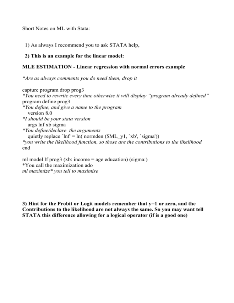
Short Notes on ML with Stata:
1) As always I recommend you to ask STATA help,
2) This is an example for the linear model:
MLE ESTIMATION - Linear regression with normal errors example
*Are as always comments you do need them, drop it
capture program drop prog3
*You need to rewrite every time otherwise it will display “program already defined”
program define prog3
*You define, and give a name to the program
version 8.0
*I should be your stata version
args lnf xb sigma
*You define/declare the arguments
quietly replace `lnf' = ln( normden ($ML_y1, `xb', `sigma'))
*you write the likelihood function, so those are the contributions to the likelihood
end
ml model lf prog3 (xb: income = age education) (sigma:)
*You call the maximization ado
ml maximize* you tell to maximise
3) Hint for the Probit or Logit models remember that y=1 or zero, and the
Contributions to the likelihood are not always the same. So you may want tell
STATA this difference allowing for a logical operator (if is a good one)
help ml
------------------------------------------------------------------------------
Title
[R] ml -- Maximum likelihood estimation
Syntax
ml model in interactive mode
ml model
method progname eq [eq ...] [if] [in] [weight] [,
model_options svy diparm_options]
ml model in noninteractive mode
ml model
method progname eq [eq ...] [if] [in] [weight], maximize
[model_options svy diparm_options noninteractive_options]
Noninteractive mode is invoked by specifying the maximize option.
Use
maximize when ml will be used as a subroutine of another ado-file or
program and you want to carry forth the problem, from definition to
posting of final results, in one command.
ml clear
ml query
ml check
ml search
[[/]eqname[:] #lb #ub ] [...] [, search_options]
ml plot
[eqname:]name [# [# [#]]] [, saving(filename[, replace])]
ml init
{ [eqname:]name=# | /eqname=# } [...]
ml init
# [# ...], copy
ml init
matname [, copy skip ]
ml report
ml trace
{ on | off }
ml count
[ clear | on | off ]
ml maximize [, ml_maximize_options display_options eform_option]
ml graph
[#] [, saving(filename[, replace]) ]
ml display
[, display_options eform_option]
ml footnote
where method is { lf | d0 | d1 | d1debug | d2 | d2debug },
eq is the equation to be estimated, enclosed in parentheses, and
optionally with a name to be given to the equation, preceded by a
colon,
( [eqname:] [varlist_y =] [varlist_x] [, eq_options] )
or eq is the name of a parameter, such as sigma with a slash in front
/eqname
which is equivalent to
(eqname:)
and diparm_options is one or more diparm(diparm_args) options where
diparm_args is either __sep__ or anything accepted by the
"undocumented" _diparm command; see _diparm.
eq_options
description
------------------------------------------------------------------------noconstant
offset(varname_o)
do not include an intercept in the equation
include varname_o in model with coefficient
constrained to 1
exposure(varname_e)
include ln(varname_e) in model with
coefficient constrained to 1
-------------------------------------------------------------------------
model_options
description
------------------------------------------------------------------------robust
cluster(varname)
synonym for vce(robust)
adjust standard errors for intragroup
correlation; implies robust
constraints(numlist)
constraints(matname)
constraints by number to be applied
matrix that contains the constraints to be
applied
nocnsnotes
do not display notes when constraints are
dropped
title(string)
nopreserve
place a title on the estimation output
do not preserve the estimation subsample in
memory
collinear
keep collinear variables within equations
missing
keep observations containing variables with
missing values
lf0(#k #ll)
number of parameters and log-likelihood
value of the "constant-only" model
continue
specifies that a model has been fitted and
sets the initial values b_0 for the model
to be fitted based on those results
waldtest(#)
perform a Wald test; see Options for use
with ml model in interactive or
noninteractive mode below
obs(#)
number of observations
noscvars
do not create and pass score variables to
likelihood-evaluator program; seldom used
crittype(string)
subpop(varname)
describe the criterion optimized by ml
compute estimates for the single
subpopulation
nosvyadjust
carry out Wald test as W/k distributed
F(k,d)
technique(nr)
Stata's modified Newton-Raphson (NR)
algorithm
technique(bhhh)
Berndt-Hall-Hall-Hausman (BHHH) algorithm
technique(dfp)
Davidon-Fletcher-Powell (DFP) algorithm
technique(bfgs)
Broyden-Fletcher-Goldfarb-Shanno (BFGS)
algorithm
vce(oim)
estimate using the observed information
matrix
vce(opg)
estimate using the outer product of the
coefficient gradients
vce(robust)
compute standard errors using the
robust/sandwich estimator
-------------------------------------------------------------------------
noninteractive_options
description
------------------------------------------------------------------------init(ml_init_args)
set the initial values b_0
search(on)
equivalent to ml search, repeat(0); the
default
search(norescale)
equivalent to ml search, repeat(0)
norescale
search(quietly)
same as search(on), except that output is
suppressed
search(off)
prevents calling ml search
repeat(#)
ml search's repeat() option; see below
bounds(ml_search_bounds)
specify bounds for ml search
nowarning
suppress "convergence not achieved" message
of iterate(0)
novce
substitute the zero matrix for the variance
matrix
score(newvars)
new variables containing the contribution
to the score
maximize_options
control the maximization process; seldom
used
-------------------------------------------------------------------------
search_options
description
------------------------------------------------------------------------repeat(#)
number of random attempts to find better
initial-value vector; default is
repeat(10) in interactive mode and
repeat(0) in noninteractive mode
restart
use random actions to find starting values;
not recommended
norescale
do not rescale to improve vector parameter;
not recommended
maximize_options
control the maximization process; seldom
used
-------------------------------------------------------------------------
ml_maximize_options
description
------------------------------------------------------------------------nowarning
suppress "convergence not achieved" message
of iterate(0)
novce
substitute the zero matrix for the variance
matrix
score(newvars | stub*)
new variables containing the contribution
to the score
nooutput
suppress the display of the final results
noclear
do not clear ml problem definition after
model has converged
maximize_options
control the maximization process; seldom
used
-------------------------------------------------------------------------
display_options
description
------------------------------------------------------------------------noheader
suppress display of the header above the
coefficient table
nofootnote
suppress display of the footnote below the
coefficient table
level(#)
set confidence level; default is level(95)
first
display coefficient table reporting results
for first equation only
neq(#)
display coefficient table reporting first #
equations
plus
display coefficient table ending in
dashes-plus-sign-dashes
-------------------------------------------------------------------------
eform_option
description
------------------------------------------------------------------------eform(string)
display exponentiated coefficients; column
title is "string"
eform
display exponentiated coefficients; column
title is "exp(b)"
hr
report hazard ratios
irr
report incidence-rate ratios
or
report odds ratios
rrr
report relative risk ratios
------------------------------------------------------------------------fweights, aweights, iweights, and pweights are allowed; see weight.
With
all but method lf, you must write your likelihood-evaluation program
carefully if pweights are to be specified, and pweights may not be
specified with method d0.
See estcom for additional capabilities of estimation commands.
To
redisplay results, type ml display.
Description
ml model defines the current problem.
ml clear clears the current problem definition.
This command is rarely,
if ever, used because when you type ml model any previous problem is
automatically cleared.
ml query displays a description of the current problem.
ml check verifies that the log-likelihood evaluator you have written
works.
We strongly recommend using this command.
ml search searches for (better) initial values.
We recommend using this
command.
ml plot provides a graphical way of searching for (better) initial
values.
ml init provides a way to specify initial values.
ml report reports the values of ln L, its gradient, and its negative
Hessian at the initial values or current parameter estimates.
ml trace traces the execution of the user-defined log-likelihood
evaluation program.
ml count counts the number of times the user-defined log-likelihood
evaluation program is called; this command is seldom used.
clear clears the counter.
ml count
ml count on turns on the counter.
without arguments reports the current values of the counters.
ml count
ml count
off stops counting calls.
ml maximize maximizes the likelihood function and reports final results.
Once ml maximize has successfully completed, the previously mentioned ml
commands may no longer be used unless noclear is specified. ml graph and
ml display may be used whether or not noclear is specified.
ml graph graphs the log-likelihood values against the iteration number.
ml display redisplays final results.
ml footnote displays a warning message when the model did not converge
within the specified number of iterations.
progname is the name of a program you write to evaluate the
log-likelihood function.
In this documentation, it is referred to as the
user-written evaluator, likelihood evaluator, or sometimes simply as the
evaluator.
The program you write is written in the style required by the
method you choose.
The methods are lf, d0, d1, and d2.
Outlines of
evaluator programs for each of these methods are shown in mlmethod.
Several commands are helpful in writing a user-written evaluator for use
with ml.
See mleval for details of the mleval, mlsum, mlvecsum,
mlmatsum, and mlmatbysum commands.
Options for use with ml model in interactive or noninteractive mode
robust and cluster(varname) specify the robust variance estimator, as
does specifying pweights or the svy option.
These options will work with a method lf evaluator; all you need to
do is specify them.
These options will not work with a method d0 evaluator, and
specifying these options will result in an error message.
With method d1 or d2 evaluators in which the likelihood function
satisfies the linear-form restrictions, these options will work only
if you fill in the equation scores; otherwise, specifying these
options will result in an error message.
constraints(numlist | matname) specifies the linear constraints to be
applied during estimation.
constraints(numlist) specifies the
constraints by number. Constraints are defined using the constraint
command.
constraint(matname) specifies a matrix that contains the
constraints.
nocnsnotes prevents notes from being displayed when constraints are
dropped.
A constraint will be dropped if it is inconsistent,
contradicts other constraints, or causes some other error when the
constraint matrix is being built.
Constraints are checked in the
order they are specified.
title(string) specifies the title to be placed on the estimation output
when results are complete.
nopreserve specifies that it is not necessary for ml to ensure that only
the estimation subsample is in memory when the user-written
likelihood evaluator is called.
use method lf.
nopreserve is irrelevant when you
See [R] ml for additional details.
collinear specifies that ml not remove the collinear variables within
equations.
There is no reason you would want to leave collinear
variables in place, but this option is of interest to programmers
who, in their code, have already removed collinear variables and do
not want ml to waste computer time checking again.
missing specifies that observations containing variables with missing
values not be eliminated from the estimation sample; see [R] ml.
lf0(#k #ll) is typically used by programmers.
It specifies the number of
parameters and log-likelihood value of the "constant-only" model so
that ml can report a likelihood-ratio test rather than a Wald test.
See [R] ml for additional details.
continue is typically specified by programmers.
It does two things:
First, it specifies that a model has just been fitted by either ml or
some other estimation command, such as logit, and that the likelihood
value stored in e(ll) and the number of parameters stored in e(b) as
of this instant are the relevant values of the constant-only model.
The current value of the log likelihood is used to present a
likelihood-ratio test unless robust, cluster(), pweight, svy, or
constraints() is specified.
A likelihood-ratio test is inappropriate
when robust, cluster(), pweight, or svy is specified.
We suggest
using lrtest when constraints() is specified.
Second, continue sets the initial values b_0 for the model about to
be fitted according to the e(b) currently stored.
The comments made about specifying missing with lf0() apply equally
well in this case.
waldtest(#) is typically specified by programmers.
By default, ml
presents a Wald test, but that is overridden if options lf0() or
continue are specified.
A Wald test is performed if robust,
cluster(), or pweights are specified.
waldtest(0) prevents even the Wald test from being reported.
waldtest(-1) is the default.
It specifies that a Wald test be
performed by constraining all coefficients except for the intercept
to 0 in the first equation.
unconstrained.
Remaining equations are to be
A Wald test is performed if neither lf0() nor
continue was specified, and a Wald test is forced if robust,
cluster(), or pweights were specified.
waldtest(k) for k < -1 specifies that a Wald test be performed by
constraining all coefficients except for intercepts to 0 in the first
|k| equations; remaining equations are to be unconstrained.
A Wald
test is performed if neither lf0() nor continue was specified, and a
Wald test is forced if robust, cluster(), or pweights were specified.
waldtest(k) for k > 1 works like the options above, except that it
forces a Wald test to be reported even if the information to perform
the likelihood-ratio test is available and even if none of robust,
cluster(), or pweights were specified.
waldtest(k), k > 1, may not
be specified with lf0().
obs(#) is used mostly by programmers.
It specifies that the number of
observations reported and ultimately stored in e(N) be #.
Ordinarily, ml works that out for itself.
Programmers may want to
specify this option when, in order for the likelihood-evaluator to
work for N observations, they first had to modify the dataset so that
it contained a different number of observations.
noscvars is used mostly by programmers.
It specifies that method d0, d1,
or d2 is being used but that the likelihood-evaluation program does
not calculate or use arguments `g1', `g2', etc., which are the score
vectors.
Thus ml can save a little time by not generating and
passing those arguments.
crittype(string) is used mostly by programmers.
It allows programmers to
supply a string (up to 32 characters long) that describes the
criterion that is being optimized by ml.
The default is "log
likelihood" for nonrobust and "log pseudolikelihood" for robust
estimation.
svy indicates that ml is to pick up the svy settings set by svyset and
use the robust variance estimator.
be svyset.
This option requires the data to
svy may not be specified with weights, vce(oim|robust),
or cluster().
subpop(varname) specifies that estimates be computed for the single
subpopulation defined by the observations for which varname != 0.
Typically, varname = 1 defines the subpopulation and varname = 0
indicates observations not belonging to the subpopulation.
For
observations whose subpopulation status is uncertain, varname
should be set to missing ('.').
option.
This option requires the svy
nosvyadjust specifies that the model Wald test be carried out as W/k
distributed F(k,d), where W is the Wald test statistic, k is the
number of terms in the model excluding the constant term, d is
the total number of sampled PSUs minus the total number of
strata, and F(k,d) is an F distribution with k numerator degrees
of freedom and d denominator degrees of freedom.
adjusted Wald test is conducted:
F(k,d-k+1).
By default, an
(d-k+1)W/(kd) distributed
This option requires the svy option.
technique(algorithm_spec) specifies how the likelihood function is to be
maximized.
The following algorithms are currently implemented in ml.
For details, see the book Maximum Likelihood Estimation with Stata,
2nd Edition (Gould, Pitblado, and Sribney 2003).
technique(nr) specifies Stata's modified Newton-Raphson (NR)
algorithm.
technique(bhhh) specifies the Berndt-Hall-Hall-Hausman (BHHH)
algorithm.
technique(dfp) specifies Davidon-Fletcher-Powell (DFP) algorithm.
technique(bfgs) specifies the Broyden-Fletcher-Goldfarb-Shanno (BFGS)
algorithm.
The default is technique(nr).
You can switch between algorithms by specifying more than one in the
technique() option.
By default, ml will use an algorithm for five
iterations before switching to the next algorithm.
To specify a
different number of iterations include the number after the technique
in the option.
For example, specifying technique(bhhh 10 nr 1000)
requests that ml perform 10 iterations using the BHHH algorithm
followed by 1000 iterations using the NR algorithm, and then switch
back to BHHH for 10 iterations, and so on.
The process continues
until convergence or until the maximum number of iterations is
reached.
vce(oim|opg|robust) specifies the type of variance-covariance matrix.
This option may not be combined with the svy options.
vce(oim) specifies that the standard errors and coefficient
covariance matrix be estimated using the observed information matrix
(that is, the inverse of the negative Hessian matrix).
This is the
default for all optimization algorithms except technique(bhhh).
vce(opg) specifies that the standard errors and coefficient
covariance matrix be estimated using the outer product of the
coefficient gradients with respect to the observation likelihoods.
This is the default for technique(bhhh), except when the robust
option is supplied.
vce(robust) specifies that the standard errors and coefficient
covariance matrix be estimated using the Huber/White/sandwich
estimator.
Options for use with ml model in noninteractive mode
The following additional options are for use with ml model in
noninteractive mode.
Noninteractive mode is for programmers who use ml
as a subroutine and want to issue a single command that will carry forth
the estimation from start to finish.
maximize is required.
It specifies noninteractive mode.
init(ml_init_args) sets the initial values b_0.
ml_init_args are
whatever you would type after the ml init command.
search(on|norescale|quietly|off) specifies whether ml search is to be
used to improve the initial values.
search(on) is the default and is
equivalent to running separately ml search, repeat(0).
search(norescale) is equivalent to running separately ml search,
repeat(0) norescale.
search(quietly) is equivalent to search(on),
except that it suppresses ml search's output.
search(off) prevents
the calling of ml search altogether.
repeat(#) is ml search's repeat() option.
repeat(0) is the default.
bounds(ml_search_bounds) specifies the search bounds.
The command ml
model issues is ml search ml_search_bounds, repeat(#).
search bounds is optional.
Specifying
nowarning, novce, and score() are ml maximize's equivalent options.
maximize_options:
difficult, technique(algorithm_spec), iterate(#),
[no]log, trace, gradient, showstep, hessian, shownrtolerance,
tolerance(#), ltolerance(#), gtolerance(#), nrtolerance(#),
nonrtolerance, from(init_specs); see maximize.
These options are
seldom used.
Options for use when specifying equations
noconstant specifies that the equation not include an intercept.
offset(varname_o) specifies that the equation be xb + varname_o--that it
include varname_o with coefficient constrained to be 1.
exposure(varname_e) is an alternative to offset(varname_o); it specifies
that the equation be xb + ln(varname_e).
The equation is to include
ln(varname_e) with coefficient constrained to be 1.
Options for use with ml search
repeat(#) specifies the number of random attempts that are to be made to
find a better initial-value vector.
The default is repeat(10).
repeat(0) specifies that no random attempts be made.
More correctly,
repeat(0) specifies that no random attempts be made if the first
initial-value vector is a feasible starting point.
If it is not, ml
search will make random attempts, even if you specify repeat(0),
because it has no alternative.
The repeat() option refers to the
number of random attempts to be made to improve the initial values.
When the initial starting value vector is not feasible, ml search
will make up to 1,000 random attempts to find starting values.
It
stops the instant it finds one set of values that works and then
moves into its improve-initial-values logic.
repeat(k), k > 0, specifies the number of random attempts to be made
to improve the initial values.
restart specifies that random actions be taken to obtain starting values
and that the resulting starting values not be a deterministic
function of the current values.
Generally, you should not specify
this option because, with restart, ml search intentionally does not
produce as good a set of starting values as it could.
restart is
included for use by the optimizer when it gets into serious trouble.
The random actions ensure that the actions of the optimizer and ml
search, working together, do not result in a long, endless loop.
See
[R] ml for details.
norescale specifies that ml search not engage in its rescaling actions to
improve the parameter vector.
We do not recommend specifying this
option because rescaling tends to work so well.
maximize_options:
seldom used.
[no]log, trace; see maximize.
These options are
Option for use with ml plot
saving(filename[, replace]) specifies that the graph be saved in
filename.gph.
Options for use with ml init
copy specifies that the list of numbers or the initialization vector be
copied into the initial-value vector by position rather than by name.
skip specifies that any parameters found in the specified initialization
vector that are not also found in the model be ignored.
The default
action is to issue an error message.
Options for use with ml maximize
nowarning is allowed only with iterate(0).
"convergence not achieved" message.
nowarning suppresses the
Programmers might specify
iterate(0) nowarning when they have a vector b already containing the
final estimates and want ml to calculate the variance matrix and post
final estimation results.
In that case, specify
init(b) search(off) iterate(0) nowarning nolog.
novce is allowed only with iterate(0).
novce substitutes the zero matrix
for the variance matrix, which in effect posts estimation results as
fixed constants.
score(newvars | stub*) creates new variables containing the contributions
to the score for each equation and ancillary parameter in the model;
see [U] 20.15 Obtaining scores.
If score(newvars) is specified, the newvars must contain k new
variables, one for each equation in the model.
specified, variables named stub1, stub2, ...
If score(stub*) is
stubk are created.
The first variable contains d(ln L_j)/d(x_1j b_1); the second
variable contains d(ln L_j)/d(x_2j b_2); and so on.
nooutput suppresses display of the final results.
This is different from
prefixing ml maximize with quietly in that the iteration log is still
displayed (assuming that nolog is not specified).
noclear specifies that after the model has converged, the ml problem
definition not be cleared.
Perhaps you are having convergence
problems and intend to run the model to convergence.
If so, use ml
search to see if those values can be improved, and then start the
estimation again.
maximize_options:
difficult, iterate(#), [no]log, trace, gradient,
showstep, hessian, shownrtolerance, tolerance(#), ltolerance(#),
gtolerance(#), nrtolerance(#), nonrtolerance; see maximize.
options are seldom used.
These
display_options; see Options for use with ml display.
eform_option; see Options for use with ml display.
Option for use with ml graph
saving(filename[, replace]) specifies that the graph is to be saved in
filename.gph.
Options for use with ml display
noheader suppresses the display of the header above the coefficient table
that displays the final log-likelihood value, the number of
observations, and the model significance test.
nofootnote suppresses the display of the footnote below the coefficient
table, which displays a warning if the model fitted did not converge
within the specified number of iterations.
Use ml footnote to
display the warning (1) if you add to the coefficient table using the
plus option or (2) you have your own footnotes and want the warning
to be last.
level(#) is the standard confidence-level option.
It specifies the
confidence level, as a percentage, for confidence intervals of the
coefficients.
The default is level(95) or as set by set level; see
level.
first displays a coefficient table reporting results for the first
equation only, and the report makes it appear that the first equation
is the only equation.
This option is used by programmers who
estimate ancillary parameters in the second and subsequent equations
and who wish to report the values of such parameters themselves.
neq(#) is an alternative to first.
neq(#) displays a coefficient table
reporting results for the first # equations.
This option is used by
programmers who estimate ancillary parameters in the #+1 and
subsequent equations and who wish to report the values of such
parameters themselves.
plus displays the coefficient table, but then rather than ending the
table in a line of dashes, ends it in dashes-plus-sign-dashes.
This
is so that programmers can write additional display code to add more
results to the table and make it appear as if the combined result is
one table.
neq().
Programmers typically specify plus with options first or
This option implies nofootnote.
eform_option: eform(string), eform, hr, irr, or, and rrr display the
coefficient table in exponentiated form:
for each coefficient,
exp(b) rather than b is displayed, and standard errors and confidence
intervals are transformed.
suppressed.
Display of the intercept, if any, is
string is the table header that will be displayed above
the transformed coefficients and must be 11 characters or fewer in
length--for example, eform("Odds ratio").
The options eform, hr,
irr, or, and rrr provide a default string equivalent to "exp(b)",
"Haz.
Ratio", "IRR", "Odds Ratio", and "RRR", respectively.
These
options may not be combined.
ml display looks at e(k_eform) to determine how many equations are
affected by an eform_option; by default, only the first equation is
affected.
Examples
See [R] ml for examples.
More examples are available in Maximum
Likelihood Estimation with Stata, 3rd edition (Gould, Pitblado, and
Sribney 2006)--available from StataCorp.
Also see
Manual:
[R] ml
Online:
_estimates, matrix, maximize, ml score, mleval, nl