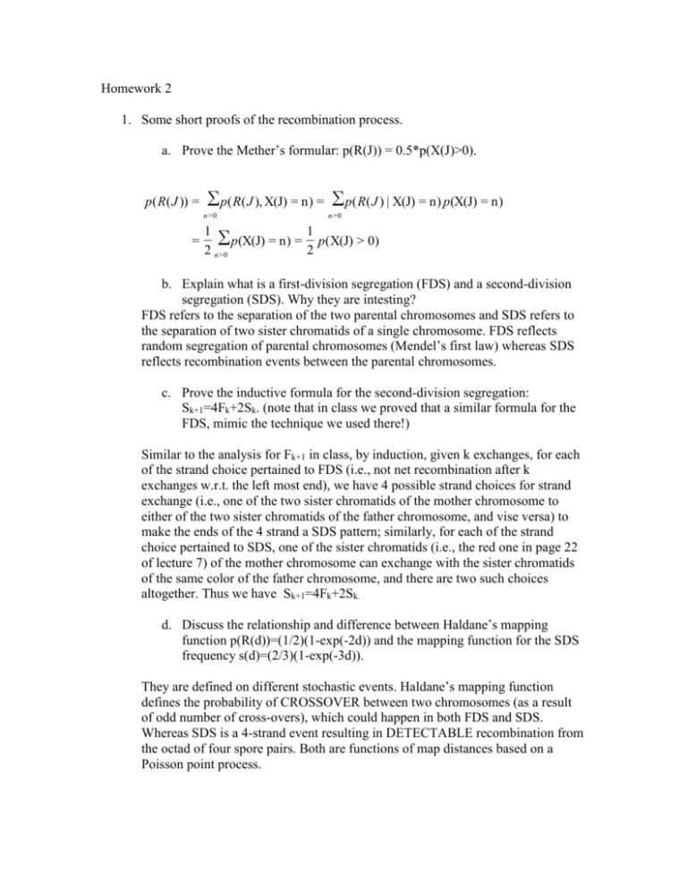
Homework 2
1. Some short proofs of the recombination process.
a. Prove the Mether’s formular: p(R(J)) = 0.5*p(X(J)>0).
p( R( J )) = ∑p( R( J ), X(J) = n ) = ∑p( R( J ) | X(J) = n ) p(X(J) = n )
n>0
=
n>0
1
1
p(X(J) = n ) = p(X(J) > 0)
∑
2 n>0
2
b. Explain what is a first-division segregation (FDS) and a second-division
segregation (SDS). Why they are intesting?
FDS refers to the separation of the two parental chromosomes and SDS refers to
the separation of two sister chromatids of a single chromosome. FDS reflects
random segregation of parental chromosomes (Mendel’s first law) whereas SDS
reflects recombination events between the parental chromosomes.
c. Prove the inductive formula for the second-division segregation:
Sk+1=4Fk+2Sk. (note that in class we proved that a similar formula for the
FDS, mimic the technique we used there!)
Similar to the analysis for Fk+1 in class, by induction, given k exchanges, for each
of the strand choice pertained to FDS (i.e., not net recombination after k
exchanges w.r.t. the left most end), we have 4 possible strand choices for strand
exchange (i.e., one of the two sister chromatids of the mother chromosome to
either of the two sister chromatids of the father chromosome, and vise versa) to
make the ends of the 4 strand a SDS pattern; similarly, for each of the strand
choice pertained to SDS, one of the sister chromatids (i.e., the red one in page 22
of lecture 7) of the mother chromosome can exchange with the sister chromatids
of the same color of the father chromosome, and there are two such choices
altogether. Thus we have Sk+1=4Fk+2Sk.
d. Discuss the relationship and difference between Haldane’s mapping
function p(R(d))=(1/2)(1-exp(-2d)) and the mapping function for the SDS
frequency s(d)=(2/3)(1-exp(-3d)).
They are defined on different stochastic events. Haldane’s mapping function
defines the probability of CROSSOVER between two chromosomes (as a result
of odd number of cross-overs), which could happen in both FDS and SDS.
Whereas SDS is a 4-strand event resulting in DETECTABLE recombination from
the octad of four spore pairs. Both are functions of map distances based on a
Poisson point process.
2. Genetic Linage Analysis
a. What does “Hardy-Weinberg equilibrium” mean in terms of inheritance
and mating outcome?
The two parental chromosomes are independently inherited, and the joint
probability factors into a product of individual probabilities.
b. Consider the following pedigree on slide 12, lecture 8:
2
1
Dd
3
5
4
dd
Dd
Dd
DD
What is the conditional probability of the genotype of the individual 2, i.e.,
p(G2=Dd|G1=Dd,G3=dd,G4=Dd,G5=DD)? Use the allele frequencies given in
the previous slides.
p(G 2 = Dd | G 1 = Dd, G 3 = dd, G 4 = Dd, G 5 = DD)
=
p(G 2 = Dd, G 1 = Dd, G 3 = dd, G 4 = Dd, G 5 = DD)
∑p(G
2
= Dd, G 1 = Dd, G 3 = dd, G 4 = Dd, G 5 = DD)
G2
∑p(G
2
= Dd, G 1 = Dd, G 3 = dd, G 4 = Dd, G 5 = DD)
G2
= (2 × .01 × .99 × .7) × (2 × .01 × .99 × .3) × (1/2 × 1/2 × .9) × (2 × 1/2 × 1/2 × .7) × (1/2 × 1/2 × .8) +
(2 × .01 × .99 × .7) × (2 × .01 × .01 × .8) × (1/2 × 0 × .9) × (1/2 × 1 × .7) × (1/2 × 1× .8)
(2 × .01 × .99 × .7) × (2 × .99 × .99 × .1) × (1/2 × 1 × .9) × (1/2 × 1 × .7) × (1/2 × 0 × .8)
p(G 2 = Dd | G 1 = Dd, G 3 = dd, G 4 = Dd, G 5 = DD) = 1
c. What LODs of linkage are additive across independent pedigrees?
Because the logarithm operation turns the joint probability from a product of
terms into a summation of the logarithms of the terms.
d. Explain for n QTLs there are 2n distinct genotypes for BC and 3n distinct
genotypes for IC?
Because for BC there are two possible genotypes for each locus (e.g., (dd, dD) or
(DD,dD)), but for IC there are three possible genotypes (i.e., (dd,DD,dD)).
3. A common strategy to infer the haplotype of multiple SNPs is to used a
parsimony criteria to evaluate the results and devise algorithm that greedily
optimize this criteria over possible solutions. Now suppose we have the genotype
of 3 SNPs of individual 1: G1={1/0, 1/0,1/0}, and we also know that the genotype
of an individual 2 is: G2={1/1, 0/0,1/1}. Can you guess what is a “parsimonious”
solution of individual 1’s haplotypes? What if G2={0/0, 0/0,0/0}?
In the first case, he will have haplotype {101/010}, in the second case, he will have
{111/000}.
a. Why haplotype is advantageous over single SNPs for linkage analysis?
It is more discriminative than SNPs, with 2n possible configurations rather than
mere binary.
b. What is the computational and biological meaning for finding “blocks” in
long sequences of SNPs?
Within a block there is low LD between SNPs, meaning that recombination
within a block is not frequent and the possible configurations of haplotypes of a
block should also be lower than expected (i.e., <<2n where n is the number of
SNPs in a block). Thus biologically this suggests block to be treated as a
recombination unit and computationally this could save the inference cost.
c. Implement the EM algorithm for Haplotype inference and test it on the
data to be posted.
To open the zipped file, use command “tar zxvf hap.data.tgz”. In the data directory, you
will see a .genos and a .haplos file. The format is as follows:
Genotype:
1603 0 2 -1 1 1 0 0 1 1 1 1 2 1 0
2103 0 -1 2 1 -1 0 0 1 -1 1 1 0 1 -1
…
The first column is the sample id, starting from the second column, you see the genotype
of 14 SNPs in each sample. “0” denote the genotype (0,0), “1” denote the genotype (1,1),
“2” denote a genotype (0,1), i.e., a heterogeneous genotype, and finally, “-1” denote an
artifact in the measurement of that SNP, and can be ignored.
Haplotype:
1603 0 0 1 -1 1 1 0 0 1 1 1 1 1 1 0
1603 1 0 0 -1 1 1 0 0 1 1 1 1 0 1 0
2103 0 0 0 1 1 1 0 0 1 -1 1 1 0 1 -1
2103 1 0 -1 0 1 0 0 0 1 1 1 1 0 1 0
…
The first column is the sample id; the second column is the index of paternal and
maternal allele; starting from the third column, you see the haplotype of 14 SNPs in each
of the two alleles of every sample. Note that “-1” denote an artifact in the measurement
of that SNP, and can be ignored.
You need to infer the haplotype of the SNPs of all the samples using your program.
Report both the haplotype and the overall error ratio (i.e., the number of wrongly inferred
loci over all heterozygous loci).