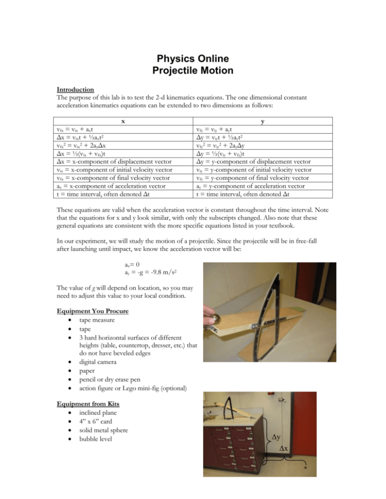
Physics Online
Projectile Motion
Introduction
The purpose of this lab is to test the 2-d kinematics equations. The one dimensional constant
acceleration kinematics equations can be extended to two dimensions as follows:
x
y
vfx = vix + axt
Δx = vixt + ½axt2
vfx2 = vix2 + 2axΔx
Δx = ½(vix + vfx)t
Δx = x-component of displacement vector
vix = x-component of initial velocity vector
vfx = x-component of final velocity vector
ax = x-component of acceleration vector
t = time interval, often denoted Δt
vfy = viy + ayt
Δy = viyt + ½ayt2
vfy2 = viy2 + 2ayΔy
Δy = ½(viy + vfy)t
Δy = y-component of displacement vector
viy = y-component of initial velocity vector
vfy = y-component of final velocity vector
ay = y-component of acceleration vector
t = time interval, often denoted Δt
These equations are valid when the acceleration vector is constant throughout the time interval. Note
that the equations for x and y look similar, with only the subscripts changed. Also note that these
general equations are consistent with the more specific equations listed in your textbook.
In our experiment, we will study the motion of a projectile. Since the projectile will be in free-fall
after launching until impact, we know the acceleration vector will be:
ax= 0
ay = -g = -9.8 m/s2
The value of g will depend on location, so you may
need to adjust this value to your local condition.
Equipment You Procure
 tape measure
 tape
 3 hard horizontal surfaces of different
heights (table, countertop, dresser, etc.) that
do not have beveled edges
 digital camera
 paper
 pencil or dry erase pen
 action figure or Lego mini-fig (optional)
Equipment from Kits
 inclined plane
 4” x 6” card
 solid metal sphere
 bubble level
Δy
Δx
Experimental Procedures
Horizontal Launch Speed Calculation
1) Select a horizontal surface. Use the bubble level to check if the surface is horizontal. If the
surface is not horizontal, then correct this or select another surface.
2) Raise the inclined plane to an angle between 20° and 45°.
3) Tape the 4”x6” card to the end of the inclined plane. An inch or two of the card should
overlap the end of the inclined plane.
4) Place the inclined plane on the horizontal surface so that the non-taped end of the card is a
few inches from the edge of the horizontal surface.
5) Measure the vertical distance between the top of the surface and the floor, Δy.
6) Place a solid metal ball at the top of the ramp and release it. It should roll down the ramp,
across the card, across the horizontal surface a couple inches, launch horizontally, and land
on the floor. Note the approximate landing place of the ball.
7) Tape down a piece of paper centered near the landing place.
8) Draw all over the metal ball so that it will make a mark on the piece of paper when it lands.
9) Roll the metal ball down the ramp again.
10) Measure the horizontal distance between the edge of the surface and the landing place, Δx.
11) Use kinematics in the y-direction to calculate the time to impact, t. You should already know
ay (assumed), viy (assumed), and Δy (measured), so use an equation that includes those three
variables plus the variable of interest, t. Note that Δy and ay will be negative using a
conventional coordinate system.
12) Use kinematics in the x-direction to calculate the launch speed, vix. You should already know
ax (assumed), Δx (measured in step 10), and t (calculated in step 11), so use an equation that
includes those three variables plus the variable of interest, vix.
Predictions of Horizontal Distances Based on Launches from Different Heights
13) Select a different horizontal surface at a significantly different height.
14) Use the bubble level to check if the surface is horizontal. If the surface is beveled or not
horizontal, then correct this or select another surface.
15) Place the inclined plane on this surface so that the non-taped end of the card is a few inches
from the edge of the horizontal surface.
16) Measure the vertical distance between the top of the surface and the floor, Δy.
17) Use kinematics in the y-direction to calculate the time to impact, t. You should already know
ay (assumed), viy (assumed), and Δy (measured in step 16), so use an equation that includes
those three variables plus the variable of interest, t. Note that Δy and ay will be negative using
a conventional coordinate system.
18) Use kinematics in the x-direction to calculate the theoretical horizontal distance, Δx. You
should already know ax (assumed), t (calculated in step 17), and vix (calculated in step 12), so
use an equation that includes those three variables plus the variable of interest, Δx.
19) Tape down a piece of paper or place your action figure at the predicted landing place.
20) Draw all over the metal ball if you are using paper.
21) Roll the solid metal ball down the ramp.
22) Note if you hit your action figure OR measure the horizontal distance between the edge of
the surface and the landing place, your experimental Δx, and compare it to your theoretical
value.
23) Repeat steps 13 through 22 with a surface of a significantly different height.
Different Launch Speed
24) Repeat steps 1 through 23 with a different ramp angle or with the ball released from
somewhere besides the top end of the ramp. This will give a different launch speed. This will
give you a total of 6 measured launches, and 4 comparisons of theoretical and experimental
distances (or 4 attempts to kill your action figure). If you do not have 6 measured launches
(2 different ramp heights x 3 different surface heights) and 4 comparisons of theory and
experiment (or 4 attempts to kill your action figure), you will have your report returned for
revision. See the following table and check that you have made all the necessary
measurements and calculations:
Measured
Ramp Angle #1
Δx (experimental)
Δy #1
Ramp Angle #1
Δx (experimental) OR note of hit/miss
Δy #2
Ramp Angle #1
Δx (experimental) OR note of hit/miss
Δy #3
Ramp Angle #2
Δx (experimental)
Δy #1
Ramp Angle #2
Δx (experimental) OR note of hit/miss
Δy #2
Ramp Angle #2
Δx (experimental) OR note of hit/miss
Δy #3
Assumed
viy
ax
ay
vix
viy
ax
ay
vix
viy
ax
ay
viy
ax
ay
vix
viy
ax
ay
vix
viy
ax
ay
Calculated
t
vix
t
Δx (theoretical)
t
Δx (theoretical)
t
vix
t
Δx (theoretical)
t
Δx (theoretical)
Notes: You do not need a graph in this report. You may skip error propagation in this lab. You must still include
error estimations for all raw data. Your conclusion will include a subjective assessment of whether or not the predictions
were “close”.