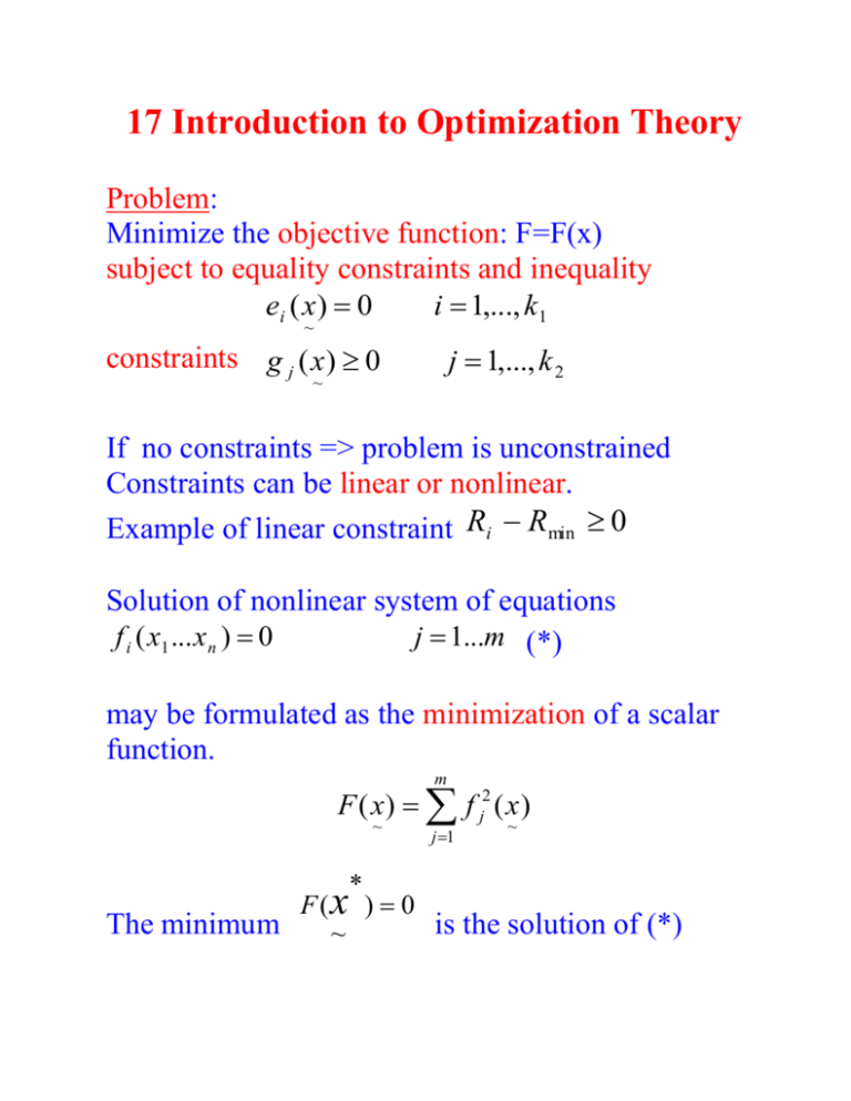
17 Introduction to Optimization Theory
Problem:
Minimize the objective function: F=F(x)
subject to equality constraints and inequality
ei ( x )  0
i  1,..., k1
~
constraints g j ( x )  0
j  1,..., k 2
~
If no constraints => problem is unconstrained
Constraints can be linear or nonlinear.
Example of linear constraint Ri  Rmin  0
Solution of nonlinear system of equations
f i ( x1 ... x n )  0
j  1...m (*)
may be formulated as the minimization of a scalar
function.
m
F ( x )   f j2 ( x )
~
*
j 1
~
F(x )  0
The minimum
is the solution of (*)
~
Most modern minimization techniques are based on
K
determining sequence of vectors X~ such that
F ( x 0 )  F ( x 1 )...  F ( x k )
~
~
~
Define gradient (points the direction of increasing f)
 F
 F   F ( x)  
~
~
~
 x1
F
F 
...
x 2
x n 


F
Condition for minimum ~ 
T
x   0
~
~ 
Lagrange multipliers method for constrained
minimization:
minimize: F ( x~ )  0
e j ( x)  0
subject to:
~
j = 1,2,. . . , k
Form the Lagrangian function
k1
Lx 1   f ( x )    j e j ( x )
j1

where   1 ,...,  k1

T
is a vector of Lagrangian
multipliers (extra variables).
 
To find the optimum of the constrained problem the
derivatives of L x ,  are set to zero
~
The
~
e j
 L F k1



0


j
xi j 1
xi
 x
L  0   i
~
~
 L  e j  x   0
  j
 ~
*
*
solution is a pair x  
~
i  1...n
j  1... k
~
17.3 Basic Iterative Algorithm

0
Given F x~ and an initial point x~ . We want to
proceed from x0 to other points such that
   F x     F x 
F x
0
1
~
k
~
~
Determine a search direction in a n-dimensional
space

s  s s
k
~
k
1

k T
n
and take a step of length dk along this direction.
Now we have
x
~
k 1
 x  dk s
k
~
~
k
In the efficient algorithm search directions must be
linearly independent, so the matrix

S s s  s
~
0
~
1
~
~
n 1

is nonsingular
Search along a line is used to determine the step
length dk using quadratic or cubic interpolation.
17.5 Quadratic Functions in Several
Variables
 
Expand F x~ into a Taylor series truncated after the
third term.


 
 x   x T F  1  x T G x  x
F
x


x

F
 
(*)
~
~
2 ~ ~ ~ ~
~
where ~ F is gradient and
 2F

 x1x1
G x   2
~ ~
  F
 x x
 n 1


is the Hessian matrix
2F
x1x 2


2F 


x1xn 

 
2
 F 

xn x n 


 
k
If we minimize F x~ in a given direction s~ then at
the minimum in this direction x~
must be orthogonal to s~
s
kT
~
(search direction)
S
k
k 1
the gradient ~ F
so
 F k 1  0
~
K
~
k 1
 F k 1
X min
(gradient)
X
K
~
^
at point x such that
 F  xˆ   0
~
We have from (*)
and
 x Gxˆ   x
T
~
~
~
~



F  x  x   F 
~
 ~

T
 1
x    x G xˆ x
~
2 ~ ~


determines type of the solution x~ .
If


G is 
~


positive definite  s G s  0  minimum
T
~
~ ~
negative definite  s G s  0  max imum
T
~
~ ~
indefinite  s G s  0 and  0  saddle po int
T
~
~ ~
Example 17.5.1
 
F x  x 2  x1   1  x1 
2
2
~
( x ) is positive definite at
Show that Hessian G
~
x̂ = [1 1]
 2
  F
 x x
G x  1 1
~ ~
  2F

 x 2 x 1
 2F 

x 1x 2 
 4  2

 
 2 2 

2

 F

x 2 x 2 
 
 
G x is positive definite since all leading principal
~ ~
minors are positive.For N  N positive definitive
i
j
matrix G~ we define s~ & s~ vectors to be G~
conjugate
s  G s  k0 0 ii  jj
i T
~
j
~ ~
i
(*)
i
s vectors satisfying (*) are also linearly
~
independent.
Example 17.5.2
Use the Hessian matrix from the previous example
and find
a) the conjugate direction to s0=[1 0]T
b) the conjugate direction to s0=[1 -1]T
To solve a), form
 4  2 1  4 
Gs  
 0   2

2
2

   
0
define s1 as s1=[a1 a2]T, we require [a1 a2][4 -2]T=0 or
a2=2 a1 so, selection of s1=[1 2]T provides the
solution. Similar in case b) we will get s1=[2 3]T
The minimum of a quadratic positive definite
function is reached in at most n iterations (n is the
number of variables).
Further properties established for the general
quadratic function
 
1 T
x Gx
~
~
~
2~ ~ ~
with positive definite matrix G~ .
F x  a  b x
T
F  b G x
The gradient is 
~
~
~ ~
Consider gradient at 2 subsequent steps:
k
k 1
 F k  b G x and
 F k 1  b G x
~
~
~ ~
~
Their difference is

   F k 1   F k  G x
k
~
~
but x~
k 1
~
~
~ ~
~
k 1
~
x k
~

 x   x  d k s k (search direction times step
~
~
k
k
  G  x  dk G s
k
size) so
F
~
k 1
k
~
~
k
~ ~
  F k  dk G s k
and
~
~
~
where the step size dk is selected to reach the
minimum in a given search direction. Multiply both
sides by a G conjugated vector s k 1 to get
s k 1 F k 1  s k 1 F k  d k s k 1 G s k  0
~
~
~
Repeating this for different k=1,…,n we can
establish that at after n steps
Fn  0
~
which concludes that the minimum of a quadratic
positive definite function is found in at most n
iterations.
17.6 Descent Methods for Minimization
The problem is how to find the search direction s~
k
A. Steepest Descent Method
s k  F k
has a tendency to oscillate
B. Conjugate Gradient Method.
s 0  F 0
s1  F 1  K11s 0
.
.
k
s  F   K ik s i1 , 1  k  n  1
k
k
i 1
where (assuming that the minimum in previous
search direction was reached) we can show that

F  F

F  F
i T
K ii
i 1 T
i
i 1
C. The Newton Method (based on 2nd derivatives)
Function F(x) is expanded into a Taylor series and
truncated to quadratic terms only
1 T k
k

k 
T
k
F x   x  F  x   x F   x G x  x ...
~
~
2 ~ ~ ~ ~
 ~ 
We want to minimize the lhs, so we differentiate this
equation wrt  x~ and set the derivative to zero to get




F k  G k x  x  0 or

~
~
~
G k x  x  F k
~
~
~
so the search direction is
  F
s x G
k
k
~
k 1
k
~
  H k F k
with Hessian matrix positive definite a full step in the
search direction can be taken
D. Variable Metric Methods
This methods are more sophisticated.
k
1. Calculate ~ F and find the search direction
s   H  Fk
k
~
k
~
where the matrix
H 1
0
~
~
~
H
~
k
is positive definite - initially
k
Only when the minimum is reached H~ simulates the
Hessian or its inverse (and then the variable metric
method looks like the Newton method).
2. Find the minimum in the search direction sk ,
determining dk and then calculate
k
   F k 1   F k  G x k
~
~
~
~
k
3. Update matrix H
~ using a formula
H
~
k 1
k
k
k
,  x ,  
 F    ,  k , H
~
~
~ 

where
H k 1  F

T

 H    x  xT
 , , H,  x,     H  1   ~ ~ ~  ~ ~ 




T
T
~
~ ~
~

x  x 

~
~
~ 
~

1

T
H


H

 k H  ~ ~ ~ ~  xT 
~
~ ~
~
 x  T H  H   x T 
 ~
~
~ ~
~ 

~
T
T
0
,  are selected scalars and  x~   0,  H
~
~
~
~
k
0
H
Note that if ~ symmetrical  H
symmetrical
~
Many updating formulae have been used, which can
be derived from expression on F, e.g.
1. If k  1 and k  0 then
 x x
H H
T
T
~
~
F 1, 0, H ,  x,    H  ~ T ~  T~ ~
~
~
~ ~

x 
 H
~
~
~
~ ~
This formula was derived by Davidson, Fletcher and
Powell and is called DFP formula.
2. If k  1 and k  1 then
  T H    x  xT


1
~
T
T
F 1,1, H ,  x,    H  1  ~ T ~  ~ T ~  T  x   H   x 
~ ~
~ 
 ~ ~ ~  ~   x    x   x   ~ ~

~
~
~
~
~`


This formula was developed by Broyden, Flethcer,
Goldfarb and Shanno and is called BFGS formula.
17.7 Constrained Minimization
x
F

F
 
Minimize
 ~
 x0
e
i
subject to  ~ 
i = 1, . . . , k1
Is solved using Lagrangian:
 
 
    
T
T
L x,    F x    i e i x  Fx    e x  F x  e x 
~
~
~
~
~ ~
~ ~`
~
~ ~ 
i
where

~



  1 ... k1
 
w.r.t. x~ and ~ and set
e  e1 ... e k1
T
Differentiate L x~ , ~
derivatives to zero:
~
T
 
 L
FN x   0
x  
~
~ ~ ~
~
 ~
L  0  
L
~
~

 e x  0
~ ~
~
 
 ~
 
(*)
where

N   e1  e2 ...  ek1
~
~
~
~

 e1 e2 ek1 
..



x

x

x
1
1
1




 e
ek1 
1


 x n
x n 
We solve (*) using Newton-Raphson iteration.
Jacobian matrix equals
 2L
   L   L    x  x
~
   ~2 ~
M  ~
~
 L
 
 x

~ 
 ~
  x~  ~

 M1  N 
~

 ~ T
0 
 N
~ 
 ~
2L 

 x
~
~

2
 L 


~
~ 
where
K1
 2 ei
2F
m jl 
  i
x j x L I 1 x j x L
m jl  M 1
and the Newton-Raphon iteration is formulated as
 xk 
   F k  N k k 
k
~

M  ~ k     Lk   ~
k
~
~


e




~
 ~ 


The first equation can be reduced since if
 k   k 1  k we have
k
k
k 1
k
k
k
M  x  N      F k  N 
~
~

  x
and  N
~
~
~
k T
~

~
k
e
~
~
~
k
~
so the iterations can be obtained from
 Mk
 ~1
 N k
 ~
 
k
 N   x k    F k 
~ 
 k~1    ~ k 
0   ~   e~ 
~

Example
In symbolic value detection problem we need to
solve the following equation to find Hs1 and Hs2
vectors:
 c   ~s 1  R11R2 ~s 2   pinv C~s 1 C1 (**)
Since  ~s 1 and  ~s 2 cannot be uniquely defined, one
can either set  ~s 2 to zero and H ~  H or introduce
s1
c
another constraint for elements of  ~s 1 and  ~s 2 , for
instance minimize the norm of H under constraint
defined by (**). The constraint minimization
problem can be formulated using a Lagrangian
function with the objective:
F   h~s2i
h~s i  ~s
with constraints
e   ~s 1  R11 R2  ~s 2  pinv C~s 1 C1  0
The Lagrangian function is defined as follows:
c
LH ~s ,    F    j e j
ej  e
j 1
where c is the cardinality of Hc
In order to locate the optimum of the constrained
minimization of ||  ~s || the derivatives of L ~s ,  
with respect to H and  are set to zero
L
 F  N  0
h~s i
L
 e j H ~s   0

where

  e1
 h~s 1 
F  2 ... 
h~s n 
  
... e    
D 
c

and
,
n = s
1
where D  R1 R2
After determining derivatives of L(  ~s ,), we will
obtain
  ~s 1    
2
     0

 ~s 2   D 
which can be split into two equations
2 ~s 1    0 and
2 ~s 2  D   0



2

~


D
 ~s 1
~
then
s 1 and s 2
After substituting results to (**) a new equation is
obtained as follows:
 ~s 1  DD  ~s 1  pinv C~s 1 C1  0
From which a unique solution for  ~s 1 can be
obtained


 ~s 1   1  DD
pinv C~s 1 C1
Thus, the minimum norm solution of (**) is
  ~s 1 
s    
 D  ~s 1 
 1