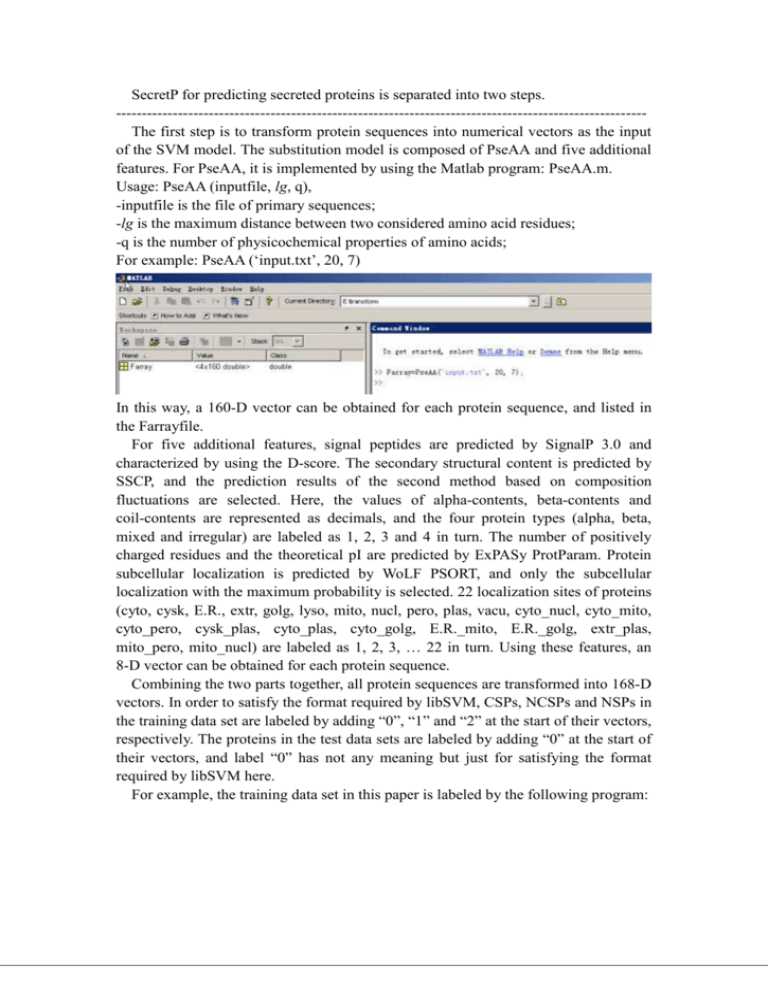
SecretP for predicting secreted proteins is separated into two steps.
------------------------------------------------------------------------------------------------------The first step is to transform protein sequences into numerical vectors as the input
of the SVM model. The substitution model is composed of PseAA and five additional
features. For PseAA, it is implemented by using the Matlab program: PseAA.m.
Usage: PseAA (inputfile, lg, q),
-inputfile is the file of primary sequences;
-lg is the maximum distance between two considered amino acid residues;
-q is the number of physicochemical properties of amino acids;
For example: PseAA (‘input.txt’, 20, 7)
In this way, a 160-D vector can be obtained for each protein sequence, and listed in
the Farrayfile.
For five additional features, signal peptides are predicted by SignalP 3.0 and
characterized by using the D-score. The secondary structural content is predicted by
SSCP, and the prediction results of the second method based on composition
fluctuations are selected. Here, the values of alpha-contents, beta-contents and
coil-contents are represented as decimals, and the four protein types (alpha, beta,
mixed and irregular) are labeled as 1, 2, 3 and 4 in turn. The number of positively
charged residues and the theoretical pI are predicted by ExPASy ProtParam. Protein
subcellular localization is predicted by WoLF PSORT, and only the subcellular
localization with the maximum probability is selected. 22 localization sites of proteins
(cyto, cysk, E.R., extr, golg, lyso, mito, nucl, pero, plas, vacu, cyto_nucl, cyto_mito,
cyto_pero, cysk_plas, cyto_plas, cyto_golg, E.R._mito, E.R._golg, extr_plas,
mito_pero, mito_nucl) are labeled as 1, 2, 3, … 22 in turn. Using these features, an
8-D vector can be obtained for each protein sequence.
Combining the two parts together, all protein sequences are transformed into 168-D
vectors. In order to satisfy the format required by libSVM, CSPs, NCSPs and NSPs in
the training data set are labeled by adding “0”, “1” and “2” at the start of their vectors,
respectively. The proteins in the test data sets are labeled by adding “0” at the start of
their vectors, and label “0” has not any meaning but just for satisfying the format
required by libSVM here.
For example, the training data set in this paper is labeled by the following program:
Here, index2file is a random matrix and used to disturb the order of data. All labeled
vectors are listed in train.txt and used as input for libSVM.
------------------------------------------------------------------------------------------------------The second step is to implement the libSVM program. The prediction result is
listed in a file, which named as: resultfile. After entering the DOS window,
---------------------------------
First, scaling the vectors in the training data set to [-1, 1] with svmscale.exe.
Usage: svmscale –l -1 –u 1 –s range inputfile > inputfile.scale
-l is the lower limit (default -1);
-u is the upper limit (default +1);
-s is the file saving scaling parameters;
-inputfile is train.txt here;
For example: svmscale –l -1 –u 1 –s range train.txt > train.scale
---------------------------------
Second, optimizing SVM parameters with grid.py.
Usage: grid.py train.scale
---------------------------------
Third, training the SVM model with svmtrain.exe. It’s notable that the data sets of
CSPs, NCSPs and NSPs are unbalanced, so different weights are assigned for them.
The number of the three types of proteins is 685, 230 and 1209, respectively. The ratio
among them is approximate to 3:1:5, and the least common multiple is 15. Therefore,
the weight for the three types of proteins is 5, 15 and 3, respectively.
Usage: svmtrain –c value1 –g value2 –wi valuei inputfile.scale modelfile
-c is the optimal regularization parameter C;
-g is the optimal kernel width parameter γ;
-wi is the weight for the i-th type of proteins;
For example: svmtrain –c 2 –g 0.125 –w0 5 –w1 15 –w2 3 train.scale model
---------------------------------
Then, scaling the vectors in the test data sets with svmscale.exe.
Usage: svmscale -r range inputfile > inputfile.scale
-r is the file restoring scaling parameters;
-inputfile is test.txt here;
---------------------------------
In the end, predicting the test data sets with svmpredict.exe.
Usage: svmpredict inputfile.scale modelfile resultfile
-----------------------------------------------------------------------------------------------------Finally, the prediction result is listed in the file: resultfile.