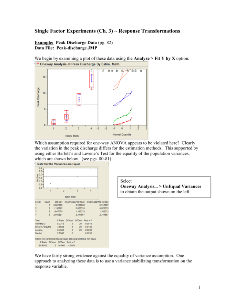
Single Factor Experiments (Ch. 3) ~ Response Transformations
Example: Peak Discharge Data (pg. 82)
Data File: Peak-discharge.JMP
We begin by examining a plot of these data using the Analyze > Fit Y by X option.
Which assumption required for one-way ANOVA appears to be violated here? Clearly
the variation in the peak discharge differs for the estimation methods. This supported by
using either Barlett’s and Levene’s Test for the equality of the population variances,
which are shown below. (see pgs. 80-81)
Select
Oneway Analysis... > UnEqual Variances
to obtain the output shown on the left.
We have fairly strong evidence against the equality of variance assumption. One
approach to analyzing these data is to use a variance stabilizing transformation on the
response variable.
1
To estimate the variance stabilizing transformation we can follow the procedure outlined
on pgs. 82-84 of your text. For this procedure we need both the mean and standard
deviation of the peak discharge readings obtained using each of the estimation methods.
In JMP select Tables > Summary and place Estim. Method in the Group box, highlight
Peak Discharge in the variable list, and then select Mean and Std Dev from the Statistics
pull-down menu.
This will create a new spreadsheet that looks like...
When we see heteroscedasticity (i.e. non-constant error variance) we can assume that the
variation in the response is proportion to the mean. This gives the model...
 y  
or in case of a single factor experiment
 yi   i  where i = 1,...,a.
If we use a power transformation of the response, y *  y  , one can show that
 y   i   1 . If we choose   1   then  y  constant . Table 3-9 on pg. 83 of your
*
*
i
i
text shows different  values and the corresponding variance stabilizing power
transformation value  . If we have replication we can use the data to empirically
estimate  and hence  .
2
Starting with
 y   i
i
and taking logs of both sides we have,
log  yi  log    log  i .
We can use data based estimates of the population means and standard deviations. For
 yi we use S i ,the sample standard deviation for factor level i, and for  i we use yi , the
sample mean for factor level i. We then perform the simple linear regression of log S i
on log yi to obtain an estimate for the slope parameter  .
To perform the procedure outlined above in JMP we first need to transform both the
means and standard deviations to the natural log scale. Next we select Analyze > Fit Y
by X with the ln(SD) in the Y box and ln(Mean) in X box.
From the Bivariate Fit pull-down menu select Fit Line.
The estimated slope of the regression line
is ˆ  .446 which suggests a   .50 . In
other words to stabilize the error variance
we use y *  y .
3
Performing the analysis using the square root of the peak discharge we have the
following.
ANOVA TABLE ( Peak Discharge )
The error variance appears to be stabilized as none of the equality of variance tests
suggest the population variances significantly differ.
Q: Can the CI’s for the difference in the
means in the square root peak discharge scale
be interpreted meaningfully?
4
Peak Discharge Data Analyzed in Design-Expert
Design-Expert Spreadsheet
ANOVA results suggest that estimation method is significant, however the residuals
plotted vs. the predicted values suggests non-constant error variance. The variance
increases with the mean, i.e. the variance appears to be proportional to some function of
the mean.
5
Design-Expert provides another means of estimating the optimal transformation for the
response called the Box-Cox method. When there is evidence of non-constant variance
or non-normal errors we can refer to results of the Box-Cox procedure for suggested
response transformation. The results of the Box-Cox procedure from Design-Expert are
shown below and the we can see that the recommended choice for response
transformation is the square root (   .50 ).
To take the square root of the peak discharge values and repeat the analysis click on the
Transform tab, choose power transformation, and set Lambda to .50 as shown below.
After transformation the residuals look fine. The ANOVA results are the same as those
shown for JMP above.
6