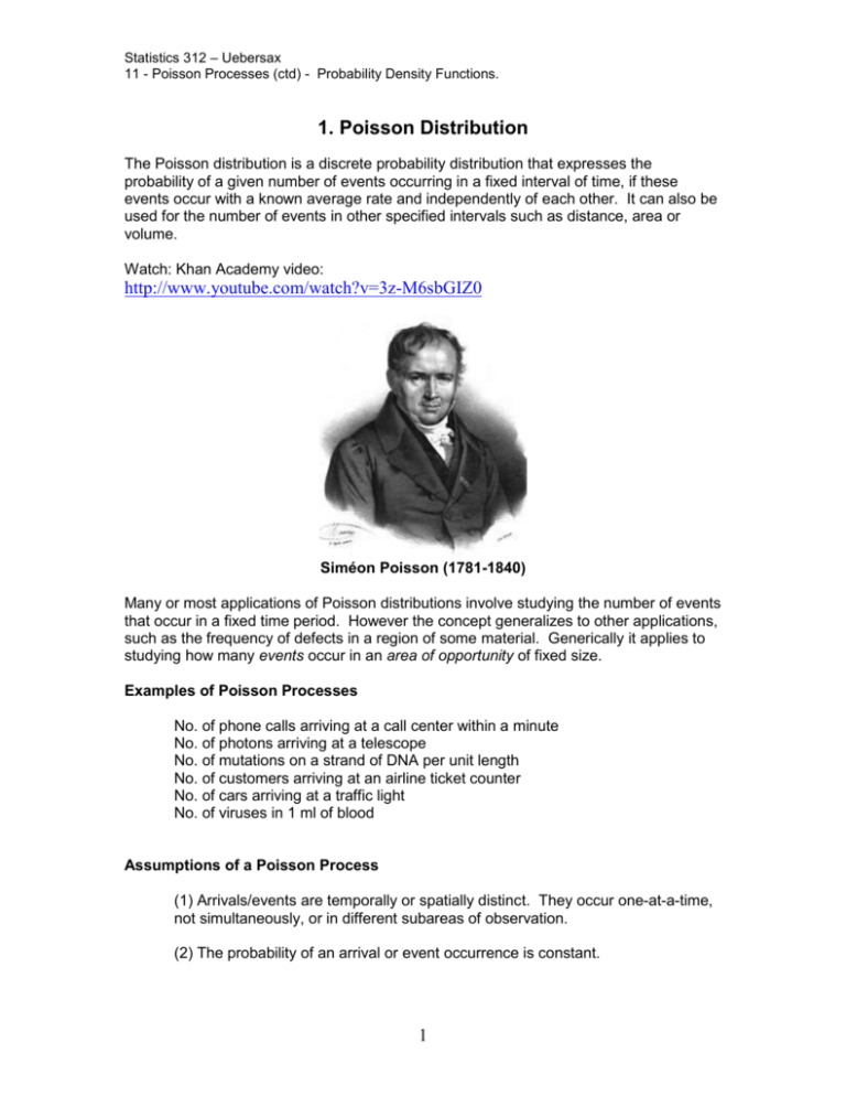
Statistics 312 – Uebersax
11 - Poisson Processes (ctd) - Probability Density Functions.
1. Poisson Distribution
The Poisson distribution is a discrete probability distribution that expresses the
probability of a given number of events occurring in a fixed interval of time, if these
events occur with a known average rate and independently of each other. It can also be
used for the number of events in other specified intervals such as distance, area or
volume.
Watch: Khan Academy video:
http://www.youtube.com/watch?v=3z-M6sbGIZ0
Siméon Poisson (1781-1840)
Many or most applications of Poisson distributions involve studying the number of events
that occur in a fixed time period. However the concept generalizes to other applications,
such as the frequency of defects in a region of some material. Generically it applies to
studying how many events occur in an area of opportunity of fixed size.
Examples of Poisson Processes
No. of phone calls arriving at a call center within a minute
No. of photons arriving at a telescope
No. of mutations on a strand of DNA per unit length
No. of customers arriving at an airline ticket counter
No. of cars arriving at a traffic light
No. of viruses in 1 ml of blood
Assumptions of a Poisson Process
(1) Arrivals/events are temporally or spatially distinct. They occur one-at-a-time,
not simultaneously, or in different subareas of observation.
(2) The probability of an arrival or event occurrence is constant.
1
Statistics 312 – Uebersax
11 - Poisson Processes (ctd) - Probability Density Functions.
(3) The probability of each arrival or event is independent of all other
arrivals/events.
The Poisson probability distribution is characterized by only one parameter,  = the
average number of events per area of opportunity.
P(X  x | )  e 

x
X = 0,1,2,..., 
x!
Example Suppose the number of flaws in a 100–foot roll of paper is a Poisson
random variable with λ = 10. Then the probability that there are eight flaws in a
100-foot roll is:
The probability of seven flaws in a 50-foot roll is:
Calculating the Poisson distribution in Excel:
POISSON(x, mu, cumulative)
x = No. of events,
mu = Average arrival/event rate (λ)
cumul = 0, noncumulative distribution
cumul = 1, cumulative distribution
Example: POISSON(8, 10, 0) = 0.112599032
Mean and the Standard Deviation of a Poisson Distribution

x = 


Example 100-foot roll:
x =  = 10
 
x
=
2
10 = 3.16
Statistics 312 – Uebersax
11 - Poisson Processes (ctd) - Probability Density Functions.
Read pp. 167–171, Prob 4.40, (a) and (c) only.
2. Probability Density Functions
Continuous random variables are variables for which any value within a specified range
can occur.
Continuous Probability Distributions
Recall what a discrete probability distribution looks like (e.g., binomial distribution)
Imagine narrower and narrower x-axis intervals, converging on infinitely narrow intervals:
i.e., a probability distribution for a continuous variable.
However, because we have infinitely many, infinitely small intervals on the x-axis, the y
axis no longer reflects probability (we'll see why shortly). Instead the y-axis is called
'probability density'.
The probability density function of x, f(x) or pdf(x), supplies the probability density (y)
for each possible value of x.
In general, for a continuous variable, the probability of x falling between a and b is:
3
Statistics 312 – Uebersax
11 - Poisson Processes (ctd) - Probability Density Functions.
P(a  X  b)  a f ( x )dx
b
Probability density function is abbreviated as pdf.
The y-axis of a pdf is rescaled so that the total area under the curve (e.g., from –inf to
+inf) is 1.0. This means the y-axis height is somewhat arbitrary. It is more or less a
scaling factor, needed to assure that the total area under the curve is 1.0.
This means that the height of pdf(x) is not the probability of x occurring. It is the
probability density of x. However the probability density is proportional to probability.
The ratio of pdf(x1) to pdf(x2) is the same as the ratio of Pr(x1) to Pr(x2).
The cumulative distribution function gives the area (probability) of being less than a
given value of x. This function is denoted as F(x) or cdf(x).
P( X  b)  F (b)  b f ( x)dx
4
Statistics 312 – Uebersax
11 - Poisson Processes (ctd) - Probability Density Functions.
The mean or expected value and variance for a continuous variable:

  E(X)   xf ( x )dx
   ( x  ) f ( x )dx
2

2

The uniform (or rectangular) distribution is a pdf where all values of x are equally likely.
We denote the lower and upper x-axis bounds as a and b, respectively. (Note: a and b
here define an entire range of possible values; above they delimited only a specific
subrange).
The expected value and variance of a uniform is given by:
5
Statistics 312 – Uebersax
11 - Poisson Processes (ctd) - Probability Density Functions.
The probability that x falls into a range defined by xlow and xhigh is:
Pr(xlow < x < xhigh) = (xhigh < x < xlow) / (b – a)
Read pp. 180–183.
6