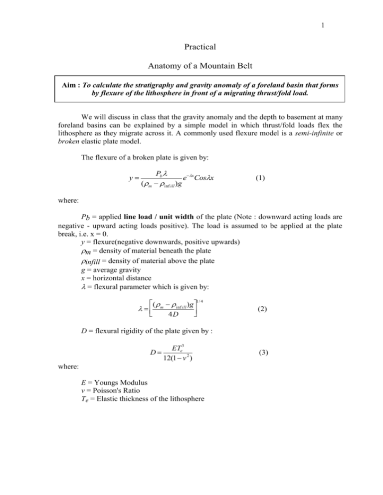
1
Practical
Anatomy of a Mountain Belt
Aim : To calculate the stratigraphy and gravity anomaly of a foreland basin that forms
by flexure of the lithosphere in front of a migrating thrust/fold load.
We will discuss in class that the gravity anomaly and the depth to basement at many
foreland basins can be explained by a simple model in which thrust/fold loads flex the
lithosphere as they migrate across it. A commonly used flexure model is a semi-infinite or
broken elastic plate model.
The flexure of a broken plate is given by:
y
Pb 
e xCosx
(m  inf ill )g
(1)
where:
Pb = 
applied line load / unit width of the plate (Note : downward acting loads are
negative - upward acting loads positive). The load is assumed to be applied at the plate
break, i.e. x = 0.
y = flexure(negative downwards, positive upwards)
m = density of material beneath the plate
infill = density of material above the plate
g = average gravity
x = horizontal distance
= flexural parameter which is given by:
(  m   inf ill )g 1/ 4
  



4D
(2)
D = flexural rigidity of the plate given by :


D
ETe3
12(1 v 2 )
where:
E = Youngs Modulus
v = Poisson'sRatio
Te = Elastic thickness of the lithosphere
(3)
2
PART 1 :
Use Excel to calculate the flexure of the lithosphere due to the load Pb,
assuming it to act on the end of a semi-infinite (i.e. broken) plate. Calculate the
flexure for values of the elastic thickness, Te, of 75, 100 and 125 km assuming the
following parameters :
m = 3330 kg m-3
infill = 2400 kg m-3
g = 9.81 m s-2
Pb = 6.0 × 1012 N m-1
v = 0.25
E = 100 GPa
Display your results on a graph.
Hint :
1. Enter the values of elastic thickness in column A. Suggestion : begin in a
row to allow for headings. Then, use Equations (3) and (2) to calculate D and
placing the results in columns B and C respectively.
2. Select a set of x values at which you want to evaluate the flexure and place
them in column B. Suggestion : begin in column A and make a list of the number of x
values, say from 0 to 15. Then, choose an x step and calculate the distance of each x
value in km. A maximum distance of 600 km should be sufficient, but allow enough
rows to add more values later.
3. Use Equation (1) to calculate the flexure for Te of 75, 100 and 125 km and
place the results in columns C, D and E respectively.
4. Plot the results on a graph showing the flexure curves as a function of
distance from the load. Click on the chart and legend and use ‘Chart’ and then ‘Chart
Options’ and ‘Source Data’ to label your graph.
3
5. Note the distance to the first point of zero flexure (i.e. the node) and plot a
graph showing the relationship between the distance to the node and Te.
PART 2 :
Use Excel to calculate the stratigraphy of a foreland basin that forms by
progressive thrust/fold loading.
Assume :
1. The basin is formed by 3 incremental loads, each of which has a value 1/3
of Pb .
2. The first load is emplaced on relatively weak lithosphere (i.e. one with Te =
75 km), the second on intermediate strength lithosphere (i.e. one with Te =
100 km) and, the third and final load on relatively strong lithosphere (i.e.
one with Te = 125 km).
3. All flexural bulges - except the one associated with the final load - are
eroded to sea-level. (Ignore the effect of any uplift that might result from
this erosion).
Hint :
1.
2.
3.
4.
5.
6.
7.
8.
9.
10.
Begin with the youngest load (i.e the one that has been emplaced
on lithosphere with Te = 125 km).
Calculate the sediment-filled flexure due to a load 1/3 of Pb
Next, consider the intermediate load (i.e the one that has been
emplaced on lithosphere with Te = 100 km).
Calculate the sediment-filled flexure due to a load 1/3 of Pb.
Erode the bulges
Calculate the depth of the sediment-filled flexure, noting that it
underlies the sediment-filled flexure of the youngest load.
End with the oldest load (i.e the one that has been emplaced on
lithosphere with Te = 75 km).
Calculate the sediment-filled flexure due to a load 1/3 of Pb
Erode the bulges
Calculate the depth of the sediment-filled flexure, noting that it
underlies the sediment-filled flexure of both the youngest and
intermediate loads.
Display the stratigraphy and label the main features.
Note: The Te values above are suggested. You can use other values if you
wish.
PART 3 :
4
Use Excel to calculate the gravity anomaly of a foreland basin that forms by
flexural loading.
Assume:
1. The density of the sediments, s, crust, c, and mantle, m, are uniform and
2600, 2800 and 3330 kg m-3 respectively.
2. The gravity anomaly can be computed using the Bouguer slab formula.
Note: The combined gravity effect of the sediment/crust and crust/mantle interfaces
(for example) using the Bouguer slab formula is :
2G(s  m )y
where G = Universal Gravitational Constant = 6.67 × 10-11 N m2 kg-2, 1 N = kg m s-2
, 1 m s-2 = 105 mGal, y = depth to the sediment/crust interface in m, s = density of
sediments = 2600 kg m-3,
and m = density of mantle = 3330 kg m-3.
PART 4 :
The final part of the practical is to use the flexure model to estimate Te of the
continental lithosphere that underlies the sub-Andean foreland basin. This basin
formed by lithospheric flexure in front of migrating loads in the sub-Andean
thrust/fold belt.
The data that you will need is posted on the web at:
http://www.earth.ox.ac.uk/~tony/watts/teaching/anatomy/resources.html
Choose any profile and download the Bouguer gravity and topography data. (It
would be good if you could choose different profiles). Import the data into Excel
(using Data, Get external data, and Import text file) and plot a profile of the
Bouguer gravity and topography.
Next, locate the plate break with respect to the mountain front. This is an
unknown parameter. You can estimate it, however, from the amount of horizontal of
shortening.
Once you have a ‘trial’ plate break, use the topography profile to estimate the
load. The load is the triangular-shaped wedge of topography located between the plate
break and the thrust front. If the height of the topography at the plate break is h and
the amount of horizontal shortening is xs, then the line load/unit width of the plate is
approximately given by :
1
hc gx s
2

5
You can use this load (which should have units of N m-1) to calculate the
flexure and, hence, Bouguer gravity anomaly for different ‘trial and error’ values of
T e.
By comparing the observed and calculated Bouguer anomaly, you should be
able to estimate the best fit Te for the profile.
Note :
1. You estimate of the magnitude of the applied load really applies to a point
mid-way in the triangular wedge – not at the plate break. This means that you
can slide the observed Bouguer gravity anomaly horizontally in order to
improve your fit.
2. The observed Bouguer gravity anomaly may not be at the correct level because
of long-wavelength contributions to the gravity field due to processes below
the flexed lithosphere (e.g. those due to mantle convection). This means that
you can slide the observed Bouguer gravity anomaly vertically in order to
improve your fit.
If time permits, repeat your calculations on another profile. Then, compare your
results to those of Watts et al (1997). A pdf of this paper can be downloaded from
:
http://www.earth.ox.ac.uk/~tony/watts/downloads/wattsetalAndes.pdf