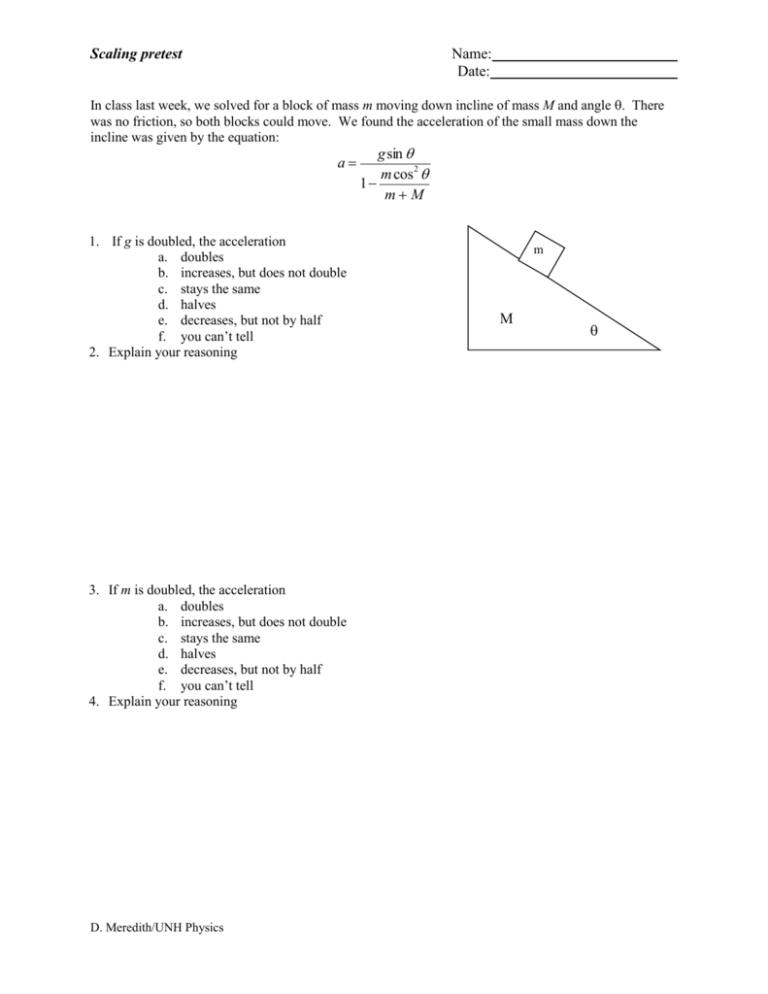
Scaling pretest
Name:
Date:
In class last week, we solved for a block of mass m moving down incline of mass M and angle . There
was no friction, so both blocks could move. We found the acceleration of the small mass down the
incline was given by the equation:
a
1. If g is doubled, the acceleration
a. doubles

b. increases, but does not double
c. stays the same
d. halves
e. decreases, but not by half
f. you can’t tell
2. Explain your reasoning
3. If m is doubled, the acceleration
a. doubles
b. increases, but does not double
c. stays the same
d. halves
e. decreases, but not by half
f. you can’t tell
4. Explain your reasoning
D. Meredith/UNH Physics
gsin 
m cos2 
1
m M
m
M

Scaling
a

5. If m and M are doubled, the acceleration
a. doubles
b. increases, but does not double
c. stays the same
d. halves
e. decreases, but not by half
f. you can’t tell
6. Explain your reasoning
D. Meredith/UNH Physics
gsin 
m cos2 
1
m M
Scaling
Tutorial overview: We often investigate how some function depends on variables (such as time
or space). But motions of a system also depend on parameters and constants. (Parameters are
values that are fixed for a single system, but will vary for different systems.) Today we will
investigate how scaling can help us gain a deeper insight into how motion depends on parameters
and constants.
a
gsin 
m cos2 
1
m M
m
M
1. What are the parameters in this equation?


2. Given the number of parameters, is it easy to plot how the acceleration depends on the
parameters?
3. We will see that scaling helps make dependence on parameters a bit less complex. There is
no procedure that always works for scaling, but one good first step is to find a parameter, or
collection of parameters, that have the same units of the key variable. Here the key variable
is acceleration, and the parameter that has units of acceleration is g. Then you introduce a
scaled acceleration:

a
g
a. If g is doubled, how does the  change? (We can imagine that we might want the
 on other planets!)
solution for this problem
b. If g is halved, how does  change?
c. Summarize: how does  depend on g?
d. What are the units of 
D. Meredith/UNH Physics
Scaling
e. Imagine that the values of the masses are fixed, and you plotted  as a function
of . You then gave this plot to Bob who lived on a planet where g=10 m/s2, and
to Sally who lived on a planet where g=20 m/s2. Will this plot be valid for both
of them? If so, what instructions would you give them to read the plot so that
they could determine the true value of acceleration of this system on their planet?
f. When plotting scaled variables we label the scaled axis as follows: acceleration in
units of g. Is this consistent with the instructions you gave to Bob and Sally? If
not, which set of directions is accurate?
g. Summary: as g changes, does the unscaled acceleration a change in complicated
ways, or does it simply stretch the same shaped function over a wider range of
values? Feel free to plot the acceleration as a function of  (take the masses to be
equal to one) with various values of g to convince yourself of your answer.
D. Meredith/UNH Physics
Scaling
4. Now let’s focus on the mass dependence. We have two masses. Let’s pick M as our mass
scale (since it’s usually the bigger mass) and define the scaled mass 

m
M
a. Write the scaled acceleration in terms of  by substituting M for m.

b. Imagine you plot () with  fixed, and hand this plot to Sally who has m=3kg
and M=15kg, and to Bob who has m=7kg and M =3.5 kg. Is the plot useful for
both of them? If so, what instructions would you give them to find the
acceleration for their system from the plot?
c. If you plotted the scaled acceleration as a function of  (with  fixed), how would
you label your  axis? Is this consistent with how we labeled the  axis?
d. Summary: as  changes, does  change in complicated ways, or does it simply
stretch the same shaped function over a wider range of values? Feel free to plot
the acceleration as a function of  for various  values to convince yourself of
your answer.
5. The final parameter is . Why is it not surprising that we have no scale for ?
D. Meredith/UNH Physics
Scaling
6. It is also possible to scale differential equations. This can be useful to gain insight before
soloving or even without solving the differential equation. Let’s take the differential
equation for a harmonic oscillator with quadratic drag.
d 2 x c dx dx k

 x 0
dt 2 m dt dt m
a. To get a foothold let’s think about the linearly damped case, where 02=k/m.

d2x
dx
 2
  02 x  0
2
dt
dt
There were three cases and three cases: underdamped, critically damped and
overdamped. Sketch x(t) for these three cases (the phase space plot is provided.)

Underdamped
Critically damped
Overdamped
b.
Are the differences between these three cases is just a matter of scale, that is, of
shrinking or enlarging the axes?
D. Meredith/UNH Physics
Scaling
c. Would you expect the same kinds of general behavior for the quadratically
damped system, that is cases where you get damped oscillations, and cases where
there are no oscillations?
d. Now let’s try to scale the quadratically damped case to see what we can learn.
What is a reasonable time scale? Hint: think of the time scale in the undamped
case.
e. Define a scaled time  similarly to the scaled acceleration. Write the differential
equation in terms of the scaled time by writing t in terms of  and the time scale;
simplify.
f. Length is the other key variable. What combination of parameters gives a length
scale? Define a scaled length w, and write the differential equation in terms of
that scaled length and simplify.
g. How does the scaled differential equation depend on parameters?
D. Meredith/UNH Physics
Scaling
h. For small damping the system oscillates. Given how the scaled differential
equation depends on parameters, do you expect oscillations even for large
damping? Explain.
i. If oscillations occur for v=0, x=1, c/m=.2, for what value of x will they occur if
v=0, c/m=200? Hint: use scaled variables.
j. For large damping the system loses energy rapidly. Given how the scaled
differential equation depends on parameters, do you expect rapid decay even for
small damping? Explain.
k. Test your expectations numerically. Don’t forget that initial conditions are given
in terms of scaled variables.
l. What have you learned from scaling about this system? In particular , what have
you learned about the phase space plots and how they change as damping is
increased? Does this system differ in important ways from the linear damping
case? What is the effect of changing the spring constant?
D. Meredith/UNH Physics