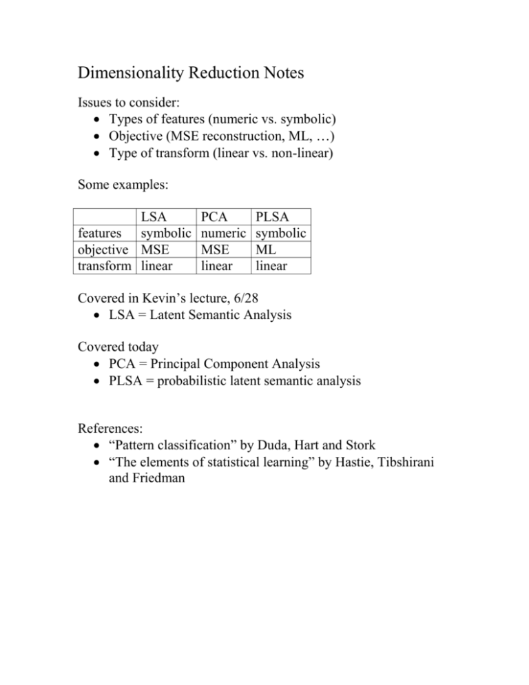
Dimensionality Reduction Notes
Issues to consider:
 Types of features (numeric vs. symbolic)
 Objective (MSE reconstruction, ML, …)
 Type of transform (linear vs. non-linear)
Some examples:
LSA
features symbolic
objective MSE
transform linear
PCA
numeric
MSE
linear
PLSA
symbolic
ML
linear
Covered in Kevin’s lecture, 6/28
 LSA = Latent Semantic Analysis
Covered today
 PCA = Principal Component Analysis
 PLSA = probabilistic latent semantic analysis
References:
 “Pattern classification” by Duda, Hart and Stork
 “The elements of statistical learning” by Hastie, Tibshirani
and Friedman
Principal Component Analysis
Interpretations:
 Orthogonal vectors in directions of greatest variance
 Basis vectors v_i that give the smallest error in
approximating x as: xhat = sum_i a_i v_i + m
Solution:
1. Given data {x_1, …, x_n} where x_i \in \Re^d
2. Compute S= sum_{k=1}^n (x_k – m)(x_k – m)^t
where m=[sum_k x_k]/n
3. Find the eigendecomposition of S (note that S is real
and symmetric)
4. Choose the d’ eigenvectors with the biggest eigenvalues
(min error approximation)
5. Reduced dimension feature vector = vector of
coefficients for the d’ principal directions:
a_i = v_i^t(x-m)
Another view:
Let X be the dxn data matrix (each column is a sample x_i) where
data is zero-mean
X = UDV^t is the singular value decomposition (SVD) of X
S = X^tX/n = VD^2V^t/n so V are the principle components &
D^2 the eigenvalues (variances in the principle directions)
Again, choose the directions with the largest singular values.
… so LSA is like PCA on word count vectors.
Probabilistic Latent Semantic Analysis
Interpretation: represent the distribution of x as a mixture and the
reduced dimension representation is the vector of mixture
component probabilities
P(x) = sum_{i=1}^m p(z_i)p(x|z_i)
mixture model
z_i = latent variables, x = vector of counts of each symbol type (M
symbols)
p(z_i) and p(x|z_i) learned using the EM algorithms, m<M
Reduced dimension representation:
y = [y_1 y_2 … y_m]^t
y_i= log p(z_i|x)
Why is this a linear transform of x???
log p(z_i|x) = log p(x|z_i) + log p(z_i) – log p(x)
(assume BOW)
= sum_j log p(x_j|z_i) + log p(z_i) – log p(x)
(assume p(x_j|z_i)=q_ij^{x_j} … unigram)
= sum_j x_j log q_ij + K_i
= x^t q_i + K_i