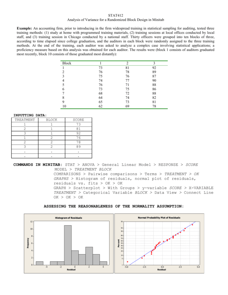
STAT412
Analysis of Variance for a Randomized Block Design in Minitab
Example: An accounting firm, prior to introducing in the firm widespread training in statistical sampling for auditing, tested three
training methods: (1) study at home with programmed training materials, (2) training sessions at local offices conducted by local
staff, and (3) training session in Chicago conducted by a national staff. Thirty officers were grouped into ten blocks of three,
according to time elapsed since college graduation, and the auditors in each block were randomly assigned to the three training
methods. At the end of the training, each auditor was asked to analyze a complex case involving statistical applications; a
proficiency measure based on this analysis was obtained for each auditor. The results were (block 1 consists of auditors graduated
most recently, block 10 consists of those graduated most distantly):
Block
1
2
3
4
5
6
7
8
9
10
INPUTTING DATA:
TREATMENT
BLOCK
1
1
2
1
3
1
1
2
2
2
3
2
.
.
.
.
1
73
76
75
74
76
73
68
64
65
62
2
81
78
76
77
71
75
72
74
73
69
3
92
89
87
90
88
86
88
82
81
78
SCORE
73
81
92
76
78
89
.
.
COMMANDS IN MINITAB: STAT > ANOVA > General Linear Model > RESPONSE > SCORE
MODEL > TREATMENT BLOCK
COMPARISONS > Pairwise comparisons > Terms > TREATMENT > OK
GRAPHS > Histogram of residuals, normal plot of residuals,
residuals vs. fits > OK > OK
GRAPH > Scatterplot > With Groups > y-variable SCORE > X-VARIABLE
TREATMENT > Categorical Variable BLOCK > Data View > Connect Line
OK > OK > OK
ASSESSING THE REASONABLENESS OF THE NORMALITY ASSUMPTION:
Normal Probability Plot of Residuals
Histogram of Residuals
12
99
10
95
90
80
70
Percent
Frequency
8
6
4
60
50
40
30
20
10
2
0
5
-4
-2
0
Residual
2
4
1
-5.0
-2.5
0.0
Residual
2.5
5.0
ASSESSING THE REASONABLENESS OF THE EQUAL VARIANCE ASSUMPTION:
Residuals Versus Fits
5.0
Residual
2.5
0.0
-2.5
-5.0
60
65
70
75
80
Fitted Value
85
90
ASSESSING THE APPROPRIATENESS OF THE NO INTERACTION ASSUMPTION:
The Scores for Each Method by Block
95
block
1
2
3
4
5
6
7
8
9
10
90
score
85
80
75
70
65
60
1
2
treat
3
Interpretation: From the appearance of the graphs, the normality and equal variance assumptions are
reasonable. There is some concern, however, about the appropriateness of the no interaction
assumption. Now we perform an analysis for a randomized block design.
Minitab Output for Performing Analysis for Randomized Block Design:
Analysis of Variance for score, using Adjusted SS for Tests
Source
treat
block
Error
Total
DF
2
9
18
29
S = 2.49815
Seq SS
1295.00
433.37
112.33
1840.70
Adj SS
1295.00
433.37
112.33
R-Sq = 93.90%
Adj MS
647.50
48.15
6.24
F
103.75
7.72
P
0.000 (H0: 1.=2.=3.)
0.000
R-Sq(adj) = 90.17%
Unusual Observations for score
Obs
5
15
score
76.0000
71.0000
Fit
71.8333
75.8333
SE Fit
1.5800
1.5800
Residual
4.1667
-4.8333
St Resid
2.15 R
-2.50 R
R denotes an observation with a large standardized residual.
H0: 1=2=3
Ha: At least two of the treatment means are different.
=.05
F=103.75
p-value=.000 < thus reject H0
Conclusion: The data provide sufficient evidence to conclude that at least two of the
treatment means are different. Now we will apply Tukey’s multiple comparisons procedure
to locate which treatment means are different.
Grouping Information Using Tukey Method and 95.0% Confidence
treat
3
2
1
N
10
10
10
Mean
86.1
74.6
70.6
Grouping
A
B
C
Means that do not share a letter are significantly different.
Tukey 95.0% Simultaneous Confidence Intervals
Response Variable score
All Pairwise Comparisons among Levels of treat
treat = 1 subtracted from:
treat
2
3
Lower
1.148
12.648
treat = 2
treat
3
Center
4.000
15.500
Upper
6.852
18.352
--------+---------+---------+-------(-----*-----)
(-----*-----)
--------+---------+---------+-------5.0
10.0
15.0
subtracted from:
Lower
8.648
Center
11.50
Upper
14.35
--------+---------+---------+-------(-----*-----)
--------+---------+---------+-------5.0
10.0
15.0