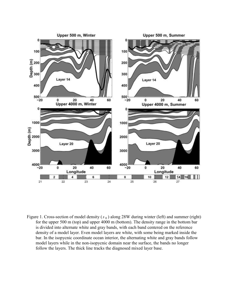
Figure 1. Cross-section of model density ( s
0
) along 28W during winter (left) and summer (right) for the upper 500 m (top) and upper 4000 m (bottom). The density range in the bottom bar is divided into alternate white and gray bands, with each band centered on the reference density of a model layer. Even model layers are white, with some being marked inside the bar. In the isopycnic coordinate ocean interior, the alternating white and gray bands follow model layers while in the non-isopycnic domain near the surface, the bands no longer follow the layers. The thick line tracks the diagnosed mixed layer base.

Figure 2. The special vertical grid used to store variables q
2
and q l for the MY mixing algorithm (right) compared to the HYCOM vertical grid (left). Interface numbers and layer numbers are shown. These two variables are stored as interface variables on the MY grid when the one-dimensional mixing algorithm is executed. They are passed as layer variables on the HYCOM grid to all other model algorithms such as horizontal advection and diffusion, and the vertical coordinate adjustment algorithm.

Figure 3. Schematic diagram of the vertical distribution of a model layer variable ( T ) for the implementation of the KT slab mixed layer model in a hybrid vertical coordinate system.
The vertical distribution of T on the left is in the model vertical coordinate system. In the vertical coordinates on the right, the model layer k containing the mixed layer base has been divided into two sublayers above and below the base with thicknesses d p
1
and d p
2
.
The value of T in the upper sublayer equals the homogenized mixed layer value. The value of T in the lower sublayer ( T
2
) is determined by the unmixing algorithm described in the text so that the thickness-weighted vertical average of sublayer T values equals the value of
T within layer k .

Figure 4. Winter mixed layer thickness (m) maps for eight 22-layer experiments.

Figure 5. Winter barotropic streamfunction (Sv) maps for eight 22-layer experiments.

Figure 6. Velocity vectors (m/s) above a reference layer chosen by inspection to reside at the base of the Ekman layer. The reference layer velocity has been subtracted from the vectors shown. Vectors are presented for two 32-layer experiments (KPP32 and MY32) and for two grid points: NAC (top) in the North Atlantic Current (Westerly wind belt), and CRBN
(bottom) in the Caribbean Sea (Trade Winds).

Figure 7. Winter surface layer temperature ( o
C) map for experiment KPP22 along with difference maps between KPP22 and seven other 22-layer experiments.

Figure 8. Winter sea surface height ( ґ 100 m) map for experiment KPP22 along with difference maps between KPP22 and seven other 22-layer experiments.

Figure 9. Winter surface heat flux (W/m
2
) map for experiment KPP22 along with difference maps between KPP22 and seven other 22-layer experiments.

Figure 10. Summer surface heat flux (W/m
2
) map for experiment KPP22 along with difference maps between KP22 and seven other 22-layer experiments.

Figure 11. Winter cross-section of s
0
for experiment KPP22 along with difference maps between KPP22 and seven other 22-layer experiments. In the isopycnic coordinate interior, differences are almost entirely the result of differences in interface depth. Above the isopycnic interior, differences within layers become large. The thick solid lines are the mixed layer base for each case while the thick dashed lines in the difference sections are the
KPP22 mixed layer base.

Figure 12. Winter temperature ( o
C) cross sections along 65W for eight 22-layer experiments.

Figure 13. Winter cross sections of zonal velocity (m/s) along the Equator for eight 22-layer experiments.

Figure 14. Winter difference maps of surface layer temperature ( o
C) between 32-layer and 22layer experiments.

Figure 15. Winter s experiments.
0 difference maps of surface layer temperature between 32-layer and 22-layer