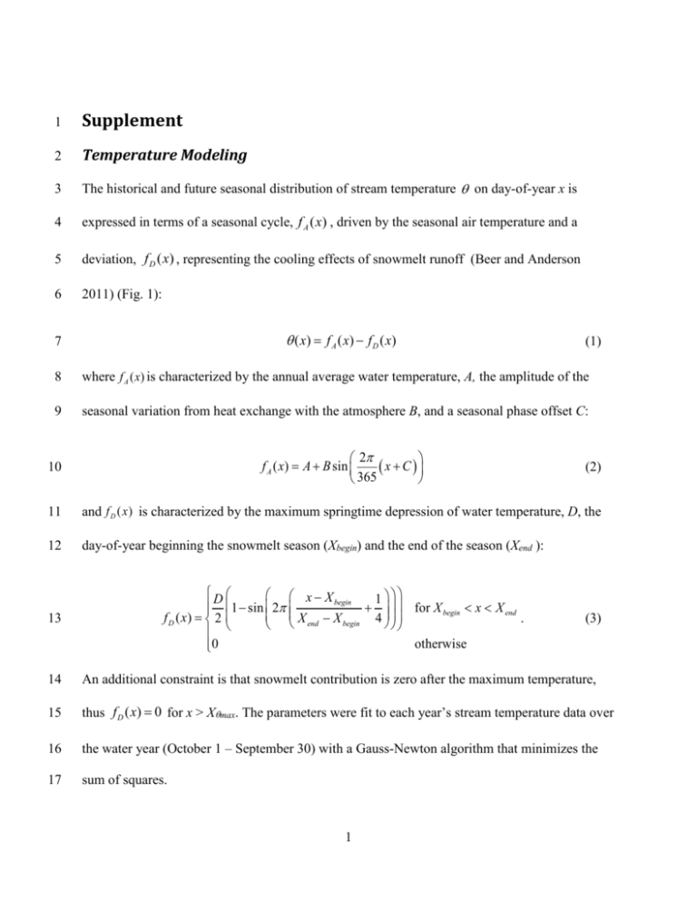
1
Supplement
2
Temperature Modeling
3
The historical and future seasonal distribution of stream temperature  on day-of-year x is
4
expressed in terms of a seasonal cycle, f A ( x) , driven by the seasonal air temperature and a
5
deviation, f D ( x) , representing the cooling effects of snowmelt runoff (Beer and Anderson
6
2011) (Fig. 1):
 ( x)  f A ( x)  f D ( x)
7
(1)
8
where f A ( x) is characterized by the annual average water temperature, A, the amplitude of the
9
seasonal variation from heat exchange with the atmosphere B, and a seasonal phase offset C:
10
 2
f A ( x)  A  B sin 
 x  C  
 365

11
and f D ( x ) is characterized by the maximum springtime depression of water temperature, D, the
12
day-of-year beginning the snowmelt season (Xbegin) and the end of the season (Xend ):
13
D 
  x  X begin
1 
    for X begin  x  X end
 1  sin  2 

f D ( x)   2 
.
  X end  X begin 4   


otherwise
0
(2)
(3)
14
An additional constraint is that snowmelt contribution is zero after the maximum temperature,
15
thus f D ( x)  0 for x > Xmax. The parameters were fit to each year’s stream temperature data over
16
the water year (October 1 – September 30) with a Gauss-Newton algorithm that minimizes the
17
sum of squares.
1
18
For each stream i, a baseline set of site-specific parameters, Pi   Ai , Bi , Ci , Di , X begin ,i , X end ,i  , was
19
estimated by fitting the model to data aggregated across all available years of stream
20
temperatures. Parameters A and D, which exhibit yearly variations, were also needed, so a set of
21
parameters was fit to water-year, y, giving site- and year-specific parameters
22
Pi , y   Ai , y , Bi , y , Ci , y , Di , y , X begin ,i , y , X end ,i , y  . Parameters A and D were then related to environmental
23
trends, and hence projected forward to mid-21st century. We assumed that the effects of climate
24
change on other parameters were small.
25
Data
26
Stream temperature data for CA, OR, WA, and ID were obtained from the United States
27
Geological Survey (http://waterdata.usgs.gov/nwis/), California Department of Water Resources,
28
Data Exchange Center (http://cdec.water.ca.gov/), and the Washington State Department of
29
Ecology (http://www.ecy.wa.gov/science/data.html). Daily water temperature values were
30
distinguished by water year (October – September) for fitting the temperature model. Several
31
sites in Washington had only monthly averages.
32
Fitting the data was an iterative process. For example, first the temperature model was fit for a
33
water year within a site (henceforth a “fit-year”). It was then inspected visually to insure that the
34
model was fitting as intended. Any conspicuously anomalous input data was excluded and if
35
model parameters were outside of existing constraints then new fitting constraints were adopted
36
and the entire procedure reapplied to all the data. By the end of the fitting process, all parameters
37
met basic constraints (e.g. 0 <  < 20, Xbegin before Xmax and both between the coolest and
38
warmest days, Xmax  Xbegin at least 50 days, etc.). All fits used here and many others are shown
39
in supplementary material (available 9 January 2013 at
2
40
http://www.cbr.washington.edu/data/Streams/data.html). An individual site had to have ≥10
41
years-worth of annual parameters so that the air and snow trends could be used to generate site-
42
specific baseline conditions to the year 2010. Missing data were tolerated as long as the six
43
parameters could be obtained.
44
Historic annual mean air temperatures (AIR) for the EPA basins were obtained from Westmap
45
(http://www.cefa.dri.edu/Westmap/). Historical SWE measures for each basin in early April were
46
compiled from Natural Resources Conservation Service SNOTEL data
47
(http://www.nrcs.usda.gov/) and California Department of Water Resources Snow Course data
48
(http://cdec.water.ca.gov/ ).
49
For incomplete series, SWE’s measured over the available years were normalized to find the in-
50
year basin anomaly, then re-computed as a basin-wide measure (Clark et al., 2001; Mote et al.,
51
2005). Normalized SWE is i , y  SWEi , y  SWE i  SWE ,i . A missing normalized value at site i in
52
year w was defined i , w 
53
then SWEi , w  i , w i  i and a basin-wide average SWE for each year y was:
54
SWE y 
55
Trend prediction
56
For historical trend estimates, available Ai , y data was related to the mean annual air temperature
57
AIRj,y across 22 EPA basins j as Ai , y  ai  bi AIR j , y   i , y . Then, air temperature trends were
58
determined as AIR j , y  c j  d j y , where y is year. The resulting projected parameter for any year


1
  j ,w where m is the number of basin sites. The missing value was
m j i
1
 SWEi , y where m is the number of basin sites i.
m i
3
59
is then Aˆi , y ( x )  ai  bi ci  bi di y and a mid-century estimate was obtained with y = 2050 (Table
60
S1).
61
Variability in Aˆi , y is assumed to remain the same as in the historic record, so up to k future
62
conditions at site i were generated using: Aˆi ,k  Aˆi   i , yk with a one-to-one mapping of the (y)
63
set of years to the k new values.
64
Di,y was developed in an analogous manner, beginning with basin-wide, annual estimates of the
65
Snow-Water Equivalent (SWE) for April 1 within basin j. To avoid negative values, basin trends
66
were derived from the log-relationship: log( SWE y )  log( )   log( y ) (Table S1) and the across-
67
year trends in Di,y , were defined Dˆ i , y   SWE j , y SWE j ,2010  Dˆ i ,2010 . In addition, Dˆ i ,2050  0 for
68
basins with insignificant snow (South Mohave, North Mohave, South Coast, North Lahontan,
69
Central Coast, San Francisco, and Oregon Basins) .
4