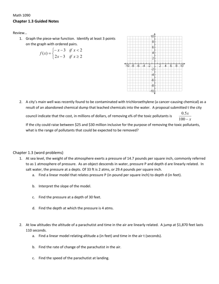
Math 1090
Chapter 1.3 Guided Notes
Review…
1. Graph the piece-wise function. Identify at least 3 points
on the graph with ordered pairs.
 x  3 if x  2
f ( x)  
 2 x  3 if x  2
2. A city’s main well was recently found to be contaminated with trichloroethylene (a cancer-causing chemical) as a
result of an abandoned chemical dump that leached chemicals into the water. A proposal submitted t the city
council indicate that the cost, in millions of dollars, of removing x% of the toxic pollutants is
0.5 x
100  x
If the city could raise between $25 and $30 million inclusive for the purpose of removing the toxic pollutants,
what is the range of pollutants that could be expected to be removed?
Chapter 1.3 (word problems)
1. At sea level, the weight of the atmosphere exerts a pressure of 14.7 pounds per square inch, commonly referred
to as 1 atmosphere of pressure. As an object descends in water, pressure P and depth d are linearly related. In
salt water, the pressure at a depts. Of 33 ft is 2 atms, or 29.4 pounds per square inch.
a. Find a linear model that relates pressure P (in pound per square inch) to depth d (in feet).
b. Interpret the slope of the model.
c. Find the pressure at a depth of 30 feet.
d. Find the depth at which the pressure is 4 atms.
2. At low altitudes the altitude of a parachutist and time in the air are linearly related. A jump at $1,870 feet lasts
110 seconds.
a. Find a linear model relating altitude a (in feet) and time in the air t (seconds).
b. Find the rate of change of the parachutist in the air.
c. Find the speed of the parachutist at landing.
3. The table lists average purchase prices for a house in an area. A linear regression model for average purchase
price is y  5.4 x  149 where x represents years since 2000 and y is average purchase price (in thousands of
dollars).
Year
2000
2001
2002
2003
2004
2005
Average Price
(in thousands)
149
154
159
165
170
176
a. Draw a scatter plot of the data and a graph of the model on the same axis.
b. Predict the average price in 2010.
c. Interpret the slope of the model.
4. Use a graphing calculator to find a linear regression model for the men’s 100 meter frestyle data given in the
table where x is years since 1980 and y is winning time (in seconds). Do the same for the women’s 100 meter
freestyle data.
Men
Women
1980
50.4
54.92
1984
49.8
55.92
1988
48.63
54.93
1992
49.02
54.65
1996
48.74
54.50
2000
48.30
53.83
2004
48.17
53.84
2008
47.38
53.12
a. Regression line for men.
b. Regression line for women.
c. Do these models indicate that the women will eventually catch up with the men?