The Multivariate Approach to the One-Way Repeated Measures ANOVA
Analyses of variance which have one or more repeated measures/within subjects factors have
a SPHERICITY ASSUMPTION (the standard error of the difference between pairs of means is
constant across all pairs of means at one level of the repeated factor versus another level of the
repeated factor. Howell discusses compound symmetry, a somewhat more restrictive assumption.
There are adjustments (of degrees of freedom) to correct for violation of the sphericity assumption,
but at a cost of lower power. A better solution might be a multivariate approach to repeated
measures designs, which does not have such a sphericity assumption.
Consider the first experiment in Karl Wuensch’s doctoral dissertation (see the article, Fostering
Animal Learning and Behavior, 20,
253-258. Wild-strain house mice were at birth cross-fostered onto house-mouse (Mus), deer mouse
(Peromyscus) or rat (Rattus) nursing mothers. Ten days after weaning each subject was tested in an
apparatus that allowed it to enter tunnels scented with clean pine shavings or with shavings bearing
the scent of Mus, Peromyscus, or Rattus. One of the variables measured was how long each subject
spent in each of the four tunnels during a twenty minute test.
house mice onto rats and deer mice: Effects on response to species odors,
The data are in the file “TUNNEL4b.DAT” and a program to do the analysis in
“MAN_RM1.SAS,” both available on my web pages. Run the program. Time spent in each tunnel is
coded in variables T_clean, T_Mus, T_Pero, and T_Rat. TT_clean, TT_Mus, TT_Pero, and TT_Rat
are these same variables after a square root transformation to normalize the within-cell distributions
and to reduce heterogeneity of variance.
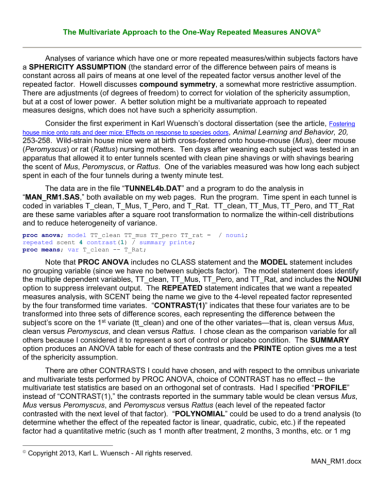
proc anova; model TT_clean TT_mus TT_pero TT_rat =
repeated scent 4 contrast(1) / summary printe;
proc means; var T_clean -- T_Rat;
/ nouni;
Note that PROC ANOVA includes no CLASS statement and the MODEL statement includes
no grouping variable (since we have no between subjects factor). The model statement does identify
the multiple dependent variables, TT_clean, TT_Mus, TT_Pero, and TT_Rat, and includes the NOUNI
option to suppress irrelevant output. The REPEATED statement indicates that we want a repeated
measures analysis, with SCENT being the name we give to the 4-level repeated factor represented
by the four transformed time variates. “CONTRAST(1)” indicates that these four variates are to be
transformed into three sets of difference scores, each representing the difference between the
subject’s score on the 1st variate (tt_clean) and one of the other variates—that is, clean versus Mus,
clean versus Peromyscus, and clean versus Rattus. I chose clean as the comparison variable for all
others because I considered it to represent a sort of control or placebo condition. The SUMMARY
option produces an ANOVA table for each of these contrasts and the PRINTE option gives me a test
of the sphericity assumption.
There are other CONTRASTS I could have chosen, and with respect to the omnibus univariate
and multivariate tests performed by PROC ANOVA, choice of CONTRAST has no effect -- the
multivariate test statistics are based on an orthogonal set of contrasts. Had I specified “PROFILE”
instead of “CONTRAST(1),” the contrasts reported in the summary table would be clean versus Mus,
Mus versus Peromyscus, and Peromyscus versus Rattus (each level of the repeated factor
contrasted with the next level of that factor). “POLYNOMIAL” could be used to do a trend analysis (to
determine whether the effect of the repeated factor is linear, quadratic, cubic, etc.) if the repeated
factor had a quantitative metric (such as 1 month after treatment, 2 months, 3 months, etc. or 1 mg
Copyright 2013, Karl L. Wuensch - All rights reserved.
MAN_RM1.docx
Page 2
dose of drug, 2 mg, 3 mg, etc.). “HELMERT” would contrast each level of the repeated factor with the
mean of all subsequent levels. “MEAN(n)” would contrast each level (except the nth) with the mean of
all other levels.
Look first at the “Sphericity Tests, Orthogonal Components” output from “PRINTE.”
Mauchly’s criterion” yields a large Chi-square with a low p value—that is, we must reject the
assumption of sphericity. If we were to use the univariate analysis we would need to adjust the
degrees of freedom for effects involving the repeated factor, scent.
The multivariate approach, “MANOVA Test Criteria for the Hypothesis of no scent Effect,”
indicates a significant effect of Scent, F(3, 33) = 7.85, p = .0004. The advantage of the multivariate
approach is that it does not require sphericity, so no adjustment for lack of sphericity is necessary.
Look at the “Univariate Tests of Hypotheses for Within Subjects Effects.” Scent has a
significant effect, F(3, 105) = 7.01, p = .0002, when we do not adjust for violation of the sphericity
assumption. To adjust, simply multiply both numerator and denominator degrees of freedom by
epsilon. Using the very conservative Greenhouse-Geisser epsilon, F(2.35, 82.15) = 7.01, p = .0009
(SAS gives the adjusted p’s).
Howell has suggested using the Huynh-Feldt epsilon rather than the more conservative
Greenhouse-Geisser when there is reason to believe that the true value of epsilon is near or above
0.75. For these data, the df using the Huynh-Feldt would be 2.53, 88.43. As you can imagine, some
so-called “expert” reviewers of manuscripts still think that df can only come in integer units, so you
might want to round to integers to avoid distressing such experts.
The “Analysis of Variance of Contrast Variables” gives the results of the planned comparisons
between the clean tunnel and each of the scented tunnels. See the untransformed means from
PROC MEANS. The mice spent significantly more time in the Mus-scented tunnel than in the clean
tunnel, F(1, 35) = 7.89, p = .0008, but the time in the clean tunnel did not differ significantly from that
in either of the other two scented tunnels. If desired, one could apply “a posteriori” tests, such as the
Tukey test, to the four means. These could be simply computed by hand, using the methods
explained in Howell and in my handout on multiple comparisons. The appropriate pooled error term
would be the MSE from the omnibus univariate ANOVA, 69.78 on 105 df. If you decided that
separate error terms would be better (a good idea when the sphericity assumption has been violated),
you could just compute correlated t-tests and use the Bonferroni or Sidak inequality to adjust
downwards the p-criterion for declaring the difference significant.
Example of Pairwise Contrasts
data multi; input block1-block3; subj = _N_;
B1vsB3 = block1-block3; B1vsB2 = block1-block2; B2vsB3=block2-block3; cards;
.......scores.......
proc means t prt; var B1vsB3 B1vsB2 B2vsB3; run;
The second part of the program includes a hypothetical set of data, the number of errors made
by each of six subjects on each of three blocks of learning trials. In addition to an omnibus analysis,
you want to make pairwise comparisons. One method is to construct a difference score for each
contrast and then use PROC MEANS to test the null that the mean difference score is zero in the
population (that is, conduct correlated t tests). Since there are only three conditions, and the omnibus
ANOVA is significant, we need not adjust the per comparison alpha.
Another method is to convert the data from a multivariate setup to a univariate setup (the
commands necessary to convert multivariate-setup data to univariate-setup data are detailed in
Chapter 16 of Cody and Smith’s Applied Statistics and the SAS Programming Language, 4th edition)
and then use one of the pairwise options on the MEANS statement of PROC ANOVA. This will allow
Page 3
you to use a pooled error term rather than individual error terms, which, as you will see, will give you
a little more power. Since we had only three conditions, I chose the LSD (Fisher) option.
Here is the code to convert to a univariate setup:
data univ; set multi;
array b[3] block1-block3; do block = 1 to 3;
errors = b[block]; output; end; drop block1-block3;
proc print; var block errors; id subj;
Look at the output from Proc Print to see how the data look after being converted to univariate
format.
SPSS: Point and Click
Obtain from my SPSS Data Page the file TUNNEL4b.sav. Bring it into SPSS. Click Analyze,
General Linear Model, Repeated Measures. In the “Within-Subject Factor Name” box, enter “scent.”
For “Number of Levels” enter “4.”
Click Add and then Define. Select t_clean, t_mus, t_pero, and t_rat (these are the transformed
variables) and scoot them into the “Within-Subjects Variables” box.
Page 4
Click Contrasts. Under “Change Contrast” select “Simple” and then select “first” for the
“Reference Category.” Click Change.
Click Continue.
Other available contrasts are “Helmert” (each level versus mean of all subsequent
levels),“Difference” (reverse Helmert, that is each level versus mean of all previous levels),
“Polynomial” (trends), Repeated (each level versus the next level), and Deviation (excepting a
reference level, each level versus the grand mean of all levels).
Click Plots. Scoot “scent” into the “Horizontal Axis” box.
Click Add, Continue.
Click Options. Scoot “scent” into the “Display means for” box. Check “Compare main effects.”
If you are afraid that the Familywise Error Boogie Man is going to get you, then change “Confidence
interval adjustment” from LSD to Bonferroni or Sidak. I’ll just take the LSD here. Under “Display”
check “Estimates of effect size.”
Page 5
Click Continue, OK.
The omnibus statistical output is essentially the same as that we got with SAS. Look at the
“Tests of Within-Subjects Effects.” The “Partial Eta-Squared” here is the scent sum of squares
divided by the (scent + error) sum of squares = 1467.267 / (1467.267 + 7326.952) = .167. Look back
at the “Multivariate Tests.” The “Partial Eta Squared” here is 1 minus Wilks lambda, 1 - .583 = .417.
While this statistic is used as a magnitude of effect estimate in MANOVA, it is clearly not what most
people think of when they think of eta-squared.
SPSS: Syntax
If you are willing to deal with the syntax of SPSS’ MANOVA utility, you can do more with your
repeated measures ANOVA than you can using the point and click interface. Here is the code to do a
one-way analysis with some special contrasts on our tunnel4b data. Assuming you already have the
data file open, all you have to do is copy and paste this code into the syntax window. If SPSS is not
already set up to open a syntax window at startup, click Edit, Options on the main SPSS window and
check “Open syntax window at start-up.” When you reboot SPSS you will get a syntax window into
which to paste commands.
manova t_clean to t_rat / wsfactors = scent(4) /
contrast(scent)=special(1,1,1,1, -3,1,1,1, 0,-2,1,1, 0,0,-1,1) /
rename=overall c_vs_mpr m_vs_pr p_vs_r / wsdesign = scent /
print=transform signif(univ) error(cor) / design /
The “wsfactors” indicates that I call the repeated factor ‘scent’ and it has 4 levels.
“contrast(scent)” is used to specify which sort of contrasts I wish to make, if any. You can choose
Page 6
from the same contrasts available with the point and click GLM analysis, or you can provide your own
special contrast coefficients, but they must be orthogonal. The first set of coefficients should be K 1’s
( where K is the number of levels of the repeated factor), then the next K-1 sets each have K
coefficients specifying the contrast you want. The set of 1’s specifies the contrast for the “overall
mean.” I then contrasted the clean tunnel with the three scented tunnels, the conspecific (Mus)
scented tunnel with the two contraspecific tunnels, and the Peromyscus tunnel with the Rattus (a
predator upon Mus) tunnel. These orthogonal contrasts actually make some sense. The rename
command was used to assign labels to the contrasts.
The wsdesign statement is optional—if omitted MANOVA assumes a full factorial model for
the within-subjects factors—if you want other than that you must specify the model you want on the
WSDESIGN statement. The design statement with no arguments produces a full factorial model with
respect to the between-subjects factors—if you want other than that you must specify the
between-subjects effects you want on the design statement.
“Print =” specifies optional output, including “transform”, the contrast transformation matrix
(inspect it to verify that the orthogonal contrasts I wanted were those computed), “signif(univ)” to
print univariate ANOVAs on the contrasts I specified, and “error(cor)” to obtain the sphericity
statistics.
With respect to omnibus univariate and multivariate tests the output is about the same we got
from SAS, only formatted differently. The univariate ANOVA on the repeated factor is called an
“Averaged F” because it is a pooled F computed with the univariate contrast ANOVA sum of squares
and degrees of freedom. Look at univariate statistics and verify that the AVERAGED SCENT SS =
the sum of the Hypoth. SS for C_VS_MPR, M_VS_PR, and P_VS_R. Sum the corresponding Error
SS and you obtain the AVERAGED WITHIN CELLS SS. Sum the contrast degrees of freedom (1,35
for each of 3) and you get the AVERAGED F DF (3,105). Note that the clean versus scented contrast
is not significant, the Mus versus other-rodent is (the Mus tunnel being most attractive), and the
Peromyscus versus Rattus is also significant (the Rattus tunnel not being very attractive).
Copyright 2013, Karl L. Wuensch - All rights reserved.
Date: Sun, 6 Feb 94 19:45:50 EST
Sender:
edstat-l@jse.stat.ncsu.edu
From: eklunn@aix02.ecs.rpi.edu (Neil Holger Eklund)
Subject:
Re: Huynh-Feldt epsilon—pronounce?
dfitts@u.washington.edu (Douglas Fitts) writes: How *do* you pronounce it? Hoon? Hi-un? Anyone
have a definitive answer?
I’ve allways heard it “Winn-Felt”
===============================================================
From: Elaine Rhodes <erhodes@camelot.bradley.edu>: I believe that it is pronounced something
close to “winn” or perhaps “when”.
===============================================================
From: maxwell gwynn f <mgwynn@mach1.wlu.ca>
My understanding is that it’s pronounced as Hine-Felt. I may be wrong, I may be right, I may
be crazy.
===============================================================
I was playing on the internet and came across your short piece on randomized block design and
noted the chain of emails regarding how to pronounce Huynh’s name. As I was his last student and
Page 7
we still meet for food or a drink, I think I can settle your debate. Huynh Huynh, first and last name,
are both pronounced, “Win;” it’s great fun to tell a table, “We’ll order when Huynh Huynh arrives.”
Best,
Brandon
Brandon L. Loudermilk, Education Associate, Office of Assessment
South Carolina Department of Education
April, 2012
Return to Wuensch’s Statistics Lessons Page
