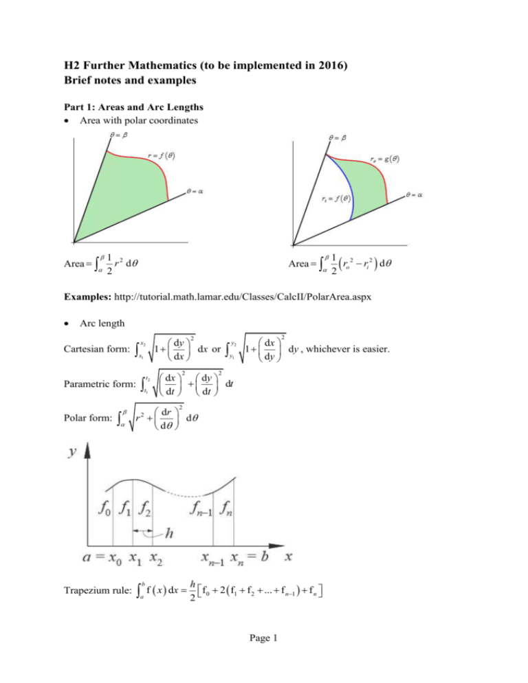
H2 Further Mathematics (to be implemented in 2016)
Brief notes and examples
Part 1: Areas and Arc Lengths
 Area with polar coordinates
Area  


1 2
r d
2
Area  




1 2
ro  ri 2 d
2
Examples: http://tutorial.math.lamar.edu/Classes/CalcII/PolarArea.aspx

Arc length
Cartesian form:
2
 dy 
1    dx or
 dx 
x2
x
1
Parametric form:
t2
t
1
Polar form:


Trapezium rule:
2
2
y2
y
1
 dx 
1    dy , whichever is easier.
 dy 
2
 dx   dy 
     dt
 dt   dt 
2
 dr 
r2  
 d
 d 
h
a f  x  dx  2 f0  2  f1  f 2  ...  f n1   f n 
b
Page 1
Simpson’s rule:
h
x f  x  dx  3 f0  4  f1  f3  ...  f n1   2  f 2  f 4  ...  f n2   f n 
xn
0
Note that n must be even.
Examples:
1. http://www.mathwords.com/a/arc_length_of_a_curve.htm
2. http://www.stewartcalculus.com/data/ESSENTIAL%20CALCULUS%20Early%20Trans
cendentals%202e/upfiles/instructor/ess_ax_0704.pdf
 Surface area of revolution
Cartesian form:
About x-axis, it is given by
x2
x
1
2
 dy 
2 y 1    dx .
 dx 
2
About y-axis, it is given by
y2
y
1
 dx 
2 x 1    dy .
 dy 
Parametric form:
About x-axis, it is given by
t2
t
1
About y-axis, it is given by
t2
t
1
2 y  t 
2
2
2
2
 dx   dy 
     dt .
 dt   dt 
 dx   dy 
2 x  t       dt .
 dt   dt 
Examples:
1. http://tutorial.math.lamar.edu/Classes/CalcII/SurfaceArea.aspx
2. http://www.phengkimving.com/calc_of_one_real_var/13_plane_curves/13_01_param_cur
ves/13_01_03_arc_len_and_area_of_surf_of_revltn_of_param_curves.htm
Part 2: Differential Equations
 Solve first-order linear DE via an integrating factor (IF)
P dx
dy
 Py  Q (P and Q are functions in x), IF is e 
For DE of the form
.
dx

Solve second-order homogeneous DE of the form a
d2 y
dy
 b  cy  0 (a, b, c are
2
dx
dx
constants)
First, solve the auxiliary equation (AE) am 2  bm  c  0 to obtain the roots m1 , m2 .
Case 1: If the roots are real and distinct, general solution (GS) is y  Aem1x  Bem2 x .
Case 2: If m1  m2  m , GS is y  emx  Ax  B  .
Case 3: If the roots are imaginary, say p  qi , GS is y  e px  A cos qx  B sin qx  .
Page 2

Solve second-order non-homogeneous DE of the form a
d2 y
dy
 b  cy  f  x 
2
dx
dx
d2 y
dy
GS has the form given by y  u  x   v  x  where u  x  is GS of a 2  b  c  0 (called
dx
dx
complementary function or CF) and v  x  is some particular integral (PI).
Case 1: f  x  is a polynomial of degree n
PI is y  an x n  an 1 x n1  ...  a1 x  a0 .
Try y  an x n 1  an1 x n  ...  a1 x 2  a0 x (when c  0 ).
The constants a0 , a1 , ..., an are found by differentiating twice and equating coefficients.
Case 2: f  x   kemx
PI is y  Pemx .
Try y  Pxemx or y  Px 2emx (when e mx is seen in CF).
The constant P is found by differentiating twice and equating coefficients.
Case 3: f  x   k1 cos rx  k2 sin rx
PI is y  p cos rx  q sin rx .
Try y  x  p cos rx  q sin rx  (when cosrx and sin rx are seen in CF).
The constants p and q are found by differentiating twice and equating coefficients.
Case 4: f  x  is the sum or difference of functions from case 1 to 3.
PI is the sum or difference of PIs from case 1 to 3.
Examples:
1. http://www.stewartcalculus.com/data/CALCULUS%20Concepts%20and%20Contexts/up
files/3c3-2ndOrderLinearEqns_Stu.pdf
2. http://www.stewartcalculus.com/data/CALCULUS%20Concepts%20and%20Contexts/up
files/3c3-NonhomgenLinEqns_Stu.pdf
 Modelling with DE
Examples:
1. http://tutorial.math.lamar.edu/Classes/DE/Modeling.aspx
2. http://www.stewartcalculus.com/data/CALCULUS%20Concepts%20and%20Contexts/up
files/3c3-AppsOf2ndOrders_Stu.pdf
Part 3: Numerical Methods
 Linear interpolation
If f  x   0 has a root between x  x1 and x  x2 , a better approximation of the root is
x3 
y2 x1  y1 x2
y1  y2
. Note: y1  f  x1  , y2  f  x2  and they have opposite signs.
Page 3

Newton-Raphson method
f  xn 
xn 1  xn 
,
f '  xn 

Iteration method
xn1  F  xn 
For example, x5  3x 2  8  0 leads to the iterative formula xn1  5 8  3xn2 .

Euler’s method to solve first-order DE y'  f  x, y 
yi 1  yi  h  f  xi , yi  where h refers to the step size.

Improved Euler formula (Heun’s method)
h
yi 1  yi  f  xi , yi   f  xi  h, yi  h  f  xi , yi   
2
Examples:
1. http://www.cimt.plymouth.ac.uk/projects/mepres/alevel/pure_ch19.pdf
2. http://mat.iitm.ac.in/home/sryedida/public_html/caimna/ode/euler/euler.html
3. http://www.math.ksu.edu/math240/book/chap1/numerical.php
Part 4: Complex Numbers


H2 Mathematics Loci and Argand diagrams
De Moivre’s theorem to find roots of z n  c and derive trigonometric identities
Examples: http://www.uea.ac.uk/jtm/6/Lec6p5.pdf
Page 4
Part 5: Loci and Conics
Page 5
Note: Eccentricity e  1 .
Page 6
Note: If a  b , we obtain a circle whose eccentricity e  0 .
Page 7
Note: Eccentricity e 
c
where c  a2  b2 . Every hyperbola has eccentricity e  1 .
a
Page 8
Note:
If A  0 or C  0 , we have a parabola.
If A and C have the same signs, we have an ellipse.
If A and C have opposite signs, we have a hyperbola.
Examples:
1. http://www.mistergmath.com/uploads/2/2/9/1/22916464/unit_10_pg_743-816.pdf
2. http://www.stewartcalculus.com/data/ESSENTIAL%20CALCULUS%20Early%20Trans
cendentals%202e/upfiles/instructor/ess_ax_0905.pdf
Part 6: Matrices and Linear Spaces
Notes and examples:
1. http://stattrek.com/tutorials/matrix-algebra-tutorial.aspx
2. http://www.maths.lse.ac.uk/personal/martin/fme2a.pdf
3. http://www.maths.lse.ac.uk/personal/martin/fme3a.pdf
4. http://www.maths.lse.ac.uk/personal/martin/fme4a.pdf
5. http://filestore.aqa.org.uk/subjects/AQA-MFP4-TEXTBOOK.PDF
6. http://web.science.mq.edu.au/~chris/matrices/CHAP07%20Diagonalisation.pdf
Page 9