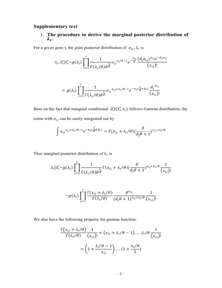
Supplementary text
1. The procedure to derive the marginal posterior distribution of
𝛌𝒊 .
For a given gene i, the joint posterior distribution of 𝑒𝑖𝑗 , λ𝑖 is
𝑐
𝜆𝑖 , ⃗⃗𝑒𝑖 |𝑥
⃗⃗⃗𝑖 ~𝑔(𝜆𝑖 ) ∏
𝑗=1
1
𝜆𝑖
Γ(𝜆𝑖 ⁄𝜃)𝜃 𝜃
𝑐
= 𝑔(𝜆𝑖 ) ∏
𝑗=1
1
𝑒𝑖𝑗
𝑒𝑖𝑗 𝜆𝑖 ⁄𝜃−1 𝑒 − 𝜃
𝑒 𝑥𝑖𝑗+𝜆𝑖 ⁄𝜃−1 𝑒
𝜆𝑖 𝑖𝑗
(𝑑𝑗 𝑒𝑖𝑗 )𝑥𝑖𝑗 𝑒 −𝑑𝑗 𝑒𝑖𝑗
(𝑥𝑖𝑗 )!
1
−𝑒𝑖𝑗 ( +𝑑𝑗 )
𝜃
Γ(𝜆𝑖 ⁄𝜃)𝜃 𝜃
𝑑𝑗 𝑥𝑖𝑗
(𝑥𝑖𝑗 )!
Base on the fact that marginal conditional ⃗⃗𝑒𝑖 |(𝑥
⃗⃗⃗𝑖 , 𝜆𝑖 ) follows Gamma distribution, the
terms with 𝑒𝑖𝑗 can be easily integrated out by
1
∫ 𝑒𝑖𝑗 𝑥𝑖𝑗+𝜆𝑖 ⁄𝜃−1 𝑒 −𝑒𝑖𝑗(𝜃+𝑑𝑗) = Γ(𝑥𝑖𝑗 + 𝜆𝑖 ⁄𝜃 )(
𝜃
)𝑥𝑖𝑗+𝜆𝑖 ⁄𝜃
𝑑𝑗 𝜃 + 1
Thus marginal posterior distribution of λ𝑖 is
𝑐
𝜆𝑖 |𝑥
⃗⃗⃗𝑖 ~𝑔(𝜆𝑖 ) ∏
𝑗=1
1
Γ(𝜆𝑖 ⁄𝜃)𝜃
𝑐
~𝑔(𝜆𝑖 ) ∏
𝑗=1
𝜆𝑖
𝜃
Γ(𝑥𝑖𝑗 + 𝜆𝑖 ⁄𝜃)(
𝜃
1
)𝑥𝑖𝑗+𝜆𝑖 ⁄𝜃
𝑑𝑗 𝜃 + 1
(𝑥𝑖𝑗 )!
Γ(𝑥𝑖𝑗 + 𝜆𝑖 ⁄𝜃)
𝜃 𝑥𝑖𝑗
1
Γ(𝜆𝑖 ⁄𝜃) (𝑑𝑗 𝜃 + 1)𝑥𝑖𝑗+𝜆𝑖 ⁄𝜃 (𝑥𝑖𝑗 )!
We also have the following property for gamma function:
Γ(𝑥𝑖𝑗 + 𝜆𝑖 ⁄𝜃) 1
1
= (𝑥𝑖𝑗 + 𝜆𝑖 ⁄𝜃 − 1) … . 𝜆𝑖 ⁄𝜃
Γ(𝜆𝑖 ⁄𝜃) (𝑥𝑖𝑗 )!
(𝑥𝑖𝑗 )!
= (1 +
𝜆𝑖 ⁄𝜃 − 1
𝜆𝑖 ⁄𝜃
) … . (1 +
)
𝑥𝑖𝑗
1
-1-
𝑥𝑖𝑗
= ∏(1 +
𝑘=1
𝜆𝑖 ⁄𝜃 − 1
)
𝑘
Thus the log transformed marginal posterior distribution of λ𝑖 is given by
𝑐
𝑥𝑖𝑗
log⁡(𝜆𝑖 |𝑥
⃗⃗⃗𝑖 )~ log(𝑔(𝜆𝑖 )) + ∑ ∑ 𝑙𝑜𝑔(1 +
𝑗=1 𝑘=1
𝜆𝑖 ⁄𝜃 − 1
) + 𝑙𝑜𝑔𝜃 ∑ 𝑥𝑖𝑗
𝑘
𝑗
𝑐
− ∑(𝑥𝑖𝑗 + 𝜆𝑖 ⁄𝜃 )𝑙𝑜𝑔(𝑑𝑗 𝜃 + 1)
𝑗=1
2. The procedure to infer the nonparametric prior distribution,
G.
Considering a cDNA library comprising M expressed genes. A RNA-seq experiment
is conducted and one sample is taken. Let 𝑥𝑖 be the number of observed reads mapped
to gene i with i = 1,2, … , N , where N is total number of observed genes. It is
important to note that N is a known number and M is unknown. Let nx denote the
number of genes with exactly x reads in the sample. Because gene i is unseen when
𝑥𝑖 = 0, n0 denotes the number of genes unseen in the sample and we have the
following equation, N = ∑∞
𝑥=1 𝑛𝑥 = 𝑀 − 𝑛0 .
Considering a gene i, it is well known that 𝑥𝑖 follows a binomial distribution and can
be approximated well by a Poisson distribution with mean λ𝑖 . Assuming a prior
mixing distribution G on 𝜆𝑖 , the 𝑥𝑖 ’s arise as a sample from a Poisson mixture and all
𝑥𝑖 ’s are iid observations from ℎ𝐺 (𝑥) = ∫ 𝑒 −𝜆 𝜆𝑥 ⁄(𝑥!)𝑑𝐺(𝜆). Here we assume G is in
an unknown nonparametric form (discrete distribution) and we are interested in
inferring it from the data.
-2-
The full likelihood of the number of genes M and the mixing distribution G is
𝑀!
L(G, M) = (𝑀−𝑁)! ∏∞
𝑥=1 𝑛𝑥 !
𝑛
𝑥
ℎ𝐺𝑀−𝑁 (0) ∏∞
𝑥=1 ℎ𝐺 (𝑥),
which is a multinomial density function. It is known that this likelihood function can
be factored into two parts,
∞
𝑛𝑥
𝑁!
ℎ𝐺 (𝑥)
𝑀
L(G, M) = ( ) ℎ𝐺𝑀−𝑁 (0)[1 − ℎ𝐺 (0)]𝑁 × ∞
∏(
)
𝑁
∏𝑥=1 𝑛𝑥 !
1 − ℎ𝐺 (0)
𝑥=1
= 𝐿1 (𝐺, 𝑀) × 𝐿2 (𝐺).
Here the likelihood 𝐿1 (𝐺, 𝑀) is from the binomial marginal distribution of N, which
depends on both G and M. The conditional distribution of 𝑥𝑖 (i = 1,2, … , N) given M
generates 𝐿2 (𝐺), which depends on G alone. Mao and Lindsay [1] identified that the
conditional log-likelihood can be reparameterized into a Q-mixture of 0-truncated
Poisson
λx
densities
as
𝑙2 (𝑄) = ∑∞
𝑥=1 nx logfQ (x),
h (x)
where, ⁡fQ (x) = 1−hG
G (0)
=
(1−e−λ )dG(λ)
∫ x!(eλ−1) dQ(λ) and dQ(λ) = ∫(1−e−η )dG(η). Thus Q-G is a one-to-one transformation.
Q also has a discrete form since the discrete form of G. The advantage of the form
𝑙2 (𝑄) is that it is standard non-parametric mixture likelihood [2] of iid observation
from a mixture of 0-truncated Poisson variable. The properties of the NPMLE (nonparametric MLE) 𝑄̂ were detailed in [3]. A numerical algorithm to infer Q was
proposed in [4] through a combination of EM (expectation-maximization) and VEM
(vertex-exchange method) algorithms. Given an initial estimate of Q, the EM
algorithm is used to increase the likelihood and the VEM is used to update the number
of support points in Q. Iterating between the EM stages and VEM stages leads to a
fast, reliable hybrid procedure [5].
-3-
References
1.
2.
3.
4.
5.
Mao CX, Lindsay BG: Tests and diagnostics for heterogeneity in the species problem.
Comput Stat Data An 2003, 41(3-4):389-398.
Lindsay BG: Mixture models : theory, geometry, and applications. Hayward,
Calif.Alexandria, Va.: Institute of Mathematical Statistics ;American Statistical
Association; 1995.
Mao CX: Predicting the conditional probability of discovering a new class. Journal
of the American Statistical Association 2004, 99(468):1108-1118.
Mao CX: Inference on the number of species through geometric lower bounds.
Journal of the American Statistical Association 2006, 101(476):1663-1670.
Bohning D: A Review of Reliable Maximum-Likelihood Algorithms for
Semiparametric Mixture-Models. J Stat Plan Infer 1995, 47(1-2):5-28.
-4-