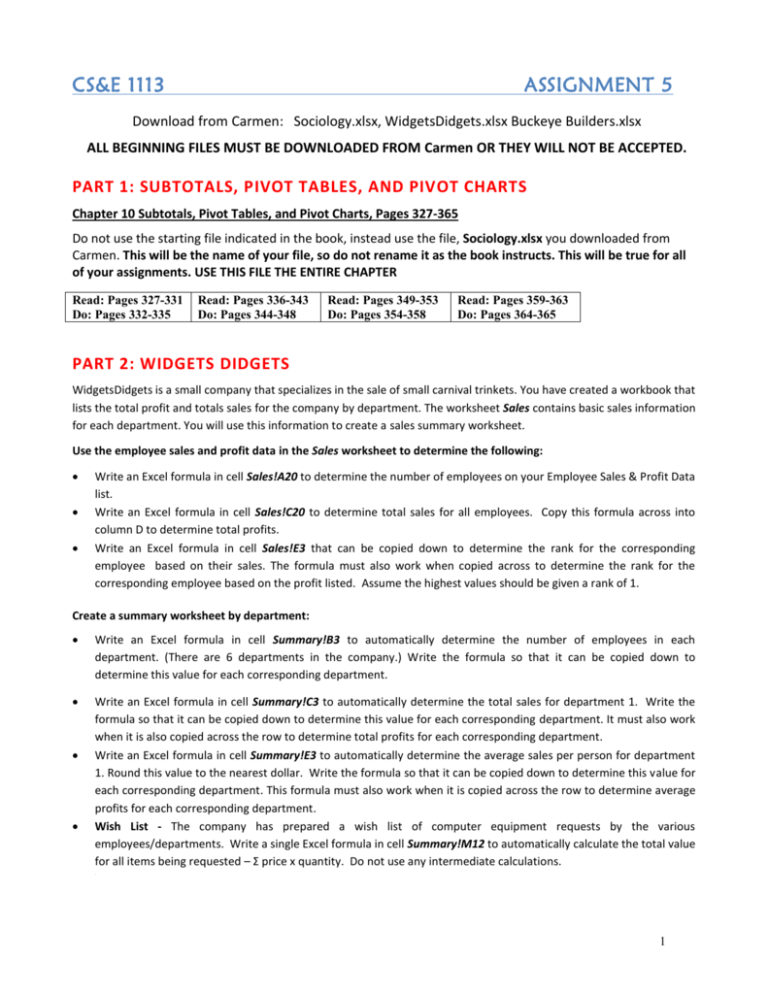
CS&E 1113
ASSIGNMENT 5
Download from Carmen: Sociology.xlsx, WidgetsDidgets.xlsx Buckeye Builders.xlsx
ALL BEGINNING FILES MUST BE DOWNLOADED FROM Carmen OR THEY WILL NOT BE ACCEPTED.
PART 1: SUBTOTALS, PIVOT TABLES, AND PIVOT CHARTS
Chapter 10 Subtotals, Pivot Tables, and Pivot Charts, Pages 327-365
Do not use the starting file indicated in the book, instead use the file, Sociology.xlsx you downloaded from
Carmen. This will be the name of your file, so do not rename it as the book instructs. This will be true for all
of your assignments. USE THIS FILE THE ENTIRE CHAPTER
Read: Pages 327-331
Do: Pages 332-335
Read: Pages 336-343
Do: Pages 344-348
Read: Pages 349-353
Do: Pages 354-358
Read: Pages 359-363
Do: Pages 364-365
PART 2: WIDGETS DIDGETS
WidgetsDidgets is a small company that specializes in the sale of small carnival trinkets. You have created a workbook that
lists the total profit and totals sales for the company by department. The worksheet Sales contains basic sales information
for each department. You will use this information to create a sales summary worksheet.
Use the employee sales and profit data in the Sales worksheet to determine the following:



Write an Excel formula in cell Sales!A20 to determine the number of employees on your Employee Sales & Profit Data
list.
Write an Excel formula in cell Sales!C20 to determine total sales for all employees. Copy this formula across into
column D to determine total profits.
Write an Excel formula in cell Sales!E3 that can be copied down to determine the rank for the corresponding
employee based on their sales. The formula must also work when copied across to determine the rank for the
corresponding employee based on the profit listed. Assume the highest values should be given a rank of 1.
Create a summary worksheet by department:

Write an Excel formula in cell Summary!B3 to automatically determine the number of employees in each
department. (There are 6 departments in the company.) Write the formula so that it can be copied down to
determine this value for each corresponding department.

Write an Excel formula in cell Summary!C3 to automatically determine the total sales for department 1. Write the
formula so that it can be copied down to determine this value for each corresponding department. It must also work
when it is also copied across the row to determine total profits for each corresponding department.
Write an Excel formula in cell Summary!E3 to automatically determine the average sales per person for department
1. Round this value to the nearest dollar. Write the formula so that it can be copied down to determine this value for
each corresponding department. This formula must also work when it is copied across the row to determine average
profits for each corresponding department.
Wish List - The company has prepared a wish list of computer equipment requests by the various
employees/departments. Write a single Excel formula in cell Summary!M12 to automatically calculate the total value
for all items being requested – Σ price x quantity. Do not use any intermediate calculations.


.
1



The company has put aside a specific amount of money $60,000 (see Summary!K14) to distribute among the
determents to allow them to purchase items from the “Wish List”. The percentage of this $60,000 each department
will be allocated based on each department’s sales as a percentage of total sales. For example, if a department’s
total sales represent 10% of the total sales for all departments, they would be allocated $6,000 (10% * $60,000) to
use towards wish list items. Write an Excel formula for cell Summary!K14 to be copied down determine the dollar
amount of the $60,000 wish list budget the corresponding department would be allocated based on the percentage
of sales earned by the corresponding department. This formula must also work when copied across to determine the
dollar amount of the wish list budget the corresponding department would be allocated if the amount is based on the
corresponding department’s profits as a percent of total profit for all departments.
Then total the new columns to see how close you’ve come to apportioning the entire budget using this method.
Write a formula in cell Summary!F13 to display the highest sales value. When copied down, this formula should
display the second and third highest sales values (respectively). This formula must also work when it is copied across
to display the highest, second highest and third highest employee profit values.
PART 3: BUCKEYE BUILDERS
In the following problem, you will be analyzing the day to day operations of a new home building company
named Buckeye Builders. One of your primary tasks will be to design an Excel workbook detailing the different
model homes they offer, the various locations available in your new development, and the customer accounts
you are currently handling.
Development Specifications
Your development area consists of 750,000 square meters of developable land. This development area already
excludes the areas for roads and a lake. You will divide the land up into as many 1/4 acre plots as possible and
build one of the model home types you offer on each plot. You may assume the development areas are
sufficiently continuous such that all of the development area will contain plots; you do not need to deduct any
area for streets and roads, etc.
Pricing Specifications
Each model home has a specific base price which is determined by the number of levels in the home and the
total square footage category of the home. The cost of the home includes the price of the base model chosen,
the plot location, and the options included. The workbook, Buckeye Builders.xlsx contains four worksheets
as follows:
Models: This worksheet outlines the specifications for the base model homes offered by the builder. It
includes all the standard features for each given model.
Base: This worksheet outlines the price in $/square foot by category for each home based on the variables just
described. Homes with less than 1,500 square feet and 1 level are priced at $85 per square foot, and $105 per
square foot for 2 levels. Homes with at least 1,500 square feet but less than 2,000 square feet are priced at
$83 per square foot for 1 level and $102 per square foot for 2 levels.
2
Units: This worksheet contains the location of the plot, the surcharge associated with the plot, the percentage
of land allocation per plot, unit conversions used for calculations, and the size of the development area
(750,000 square meters). Home buyers may be charged an additional amount depending on where on the
development they would like their home to be built. Since lake plots are the most desirable, a 50% surcharge
will be added to the total costs (base price of the home and the options total. Options explained below). So a
house with a base price + options price of $100,000 on a lake plot will cost $150,000 with the surcharge. The
surcharge for center plots is 25% and there is no surcharge for road locations. To determine the number of
each plot type, you will need the allocation percentages – the percent of the development land that is in a
specific category. For example according to the Units worksheet 15% of the land will be lake plots, 19% road
plots etc.
Customers: This worksheet describes the different options that can be added to the home, and the plot
location of the home. Options include: Jacuzzi tub in the master bedroom, walkout basement, larger plot, bay
window in dining room. Cells D4:G4 in the Customers worksheet contain the prices for each of the respective
options, which do not vary by model. If a customer has ordered this option the value TRUE will be displayed in
the corresponding cell (range D5:G12). So if a buyer chooses a Jacuzzi and bay window the corresponding cells
in columns D and G will contain TRUE values and the costs will be $4,500 plus $3,900. There are also three
different plot locations types within the development: Lake Plots (directly next to a small body of water within
the area), Center Plots (within the development away from the outer most roads surrounding the
development) and Road Plots (near the outlying boundaries of the division). There are a different numbers of
plots and different costs associated with each plot type as listed on the Units worksheet.
Now it is time to complete your analysis.
o
Based on the Total development area given in the Units worksheet, write an Excel formula in cell Units!D9
to calculate the number of Lake plots you will build per the allocation described in the Units worksheet.
This formula should also work when you copy it down to determine the number of Center plots you will
have and finally, the number of Road plots.
o
Write an Excel formula in cell Models!H3 to determine the base price for the Classic European home. This
formula should also work when you copy it down to determine the base price for the New American
Home, CSE Favorite, etc. Recall that the base price for each model depends on the number of stories and
total square footage of the home. $/SF for all combinations of stories and square footage can be found in
the Base worksheet.
o
Write an Excel formula in cell Customers!H5 to be copied down to determine the total value of the options
purchased for the first customer’s sale. When copied down, the formula will determine the total value of
options for each corresponding customer.
o
Write an Excel formula in cell Customers!I5 to be copied down to determine the Base price for the specific
model home the first customer has purchased. When copied down, the formula will determine the total
value of each home for the corresponding customer. (Do not use an IF function for this formula.)
o
Write an Excel formula in cell Customers!J5 to determine the location surcharge (not total cost), if
applicable, for the home purchased by the first customer. Remember that the surcharge percentage is
applied to the home price including options. Write the formula so that it can be copied down the column
to determine the surcharge for each corresponding customer. (Do not use an IF function for this formula.)
3
o
Write an Excel formula in cell Customers!K5 to be copied down to determine the total price of the home
that the first person will purchase. Write the formula so that it can be copied down the column to
determine the total home price for each corresponding customer. This should include options total, the
base price and location charges.
o
In order to increase the number of customers who are purchasing the various options (Jacuzzi, basement
walkout, larger plot, bay window in dining room), you have decided to offer an options package special for
a limited time- Customers who purchase all of the options listed will get the highest priced option for free.
Currently the larger plot is the most expensive option at $11,000 but keep in mind that prices are always
subject to change. Write an Excel formula for cell Customers!L5, which can be copied down the column, to
calculate the new total price of each home, taking into consideration any discounts for the options
package, if applicable.
Assignment 5 Submissions
1. Sociology.xlsx
2. WidgetsDidgets.xlsx
3. Buckeye Builders.xlsx
4