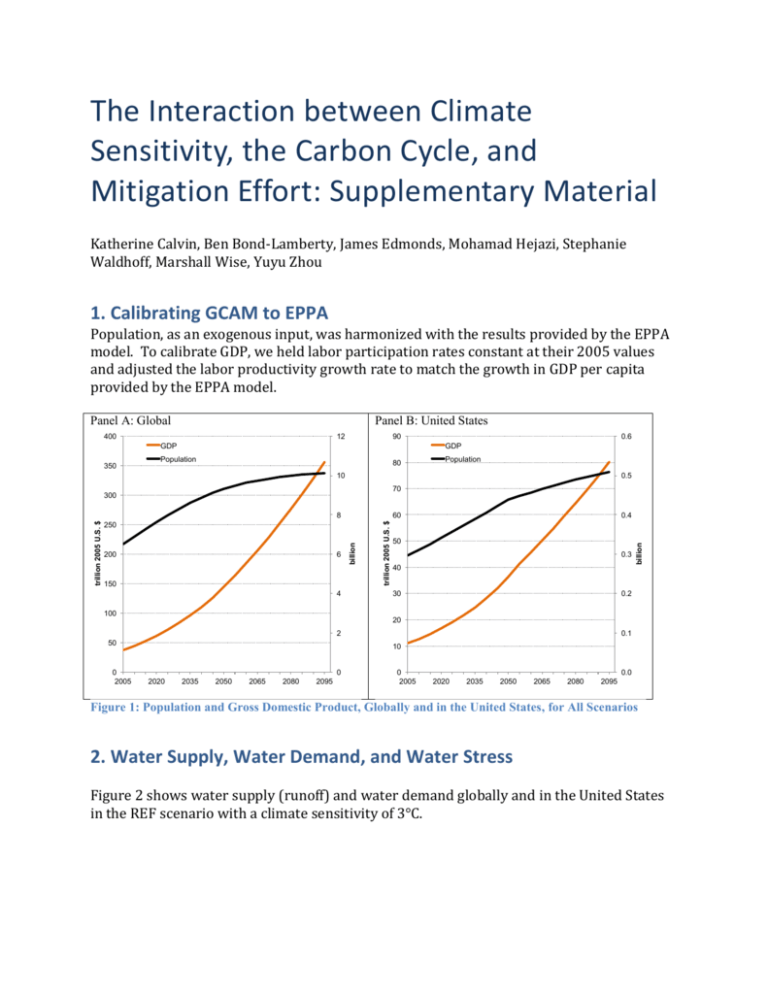
The Interaction between Climate
Sensitivity, the Carbon Cycle, and
Mitigation Effort: Supplementary Material
Katherine Calvin, Ben Bond-Lamberty, James Edmonds, Mohamad Hejazi, Stephanie
Waldhoff, Marshall Wise, Yuyu Zhou
1. Calibrating GCAM to EPPA
Population, as an exogenous input, was harmonized with the results provided by the EPPA
model. To calibrate GDP, we held labor participation rates constant at their 2005 values
and adjusted the labor productivity growth rate to match the growth in GDP per capita
provided by the EPPA model.
Panel A: Global
Panel B: United States
400
12
90
GDP
Population
80
Population
10
0.5
70
300
200
6
150
4
100
trillion 2005 U.S. $
60
billion
trillion 2005 U.S. $
8
250
0.4
50
0.3
40
30
0.2
20
2
50
0
2005
billion
350
0.6
GDP
0.1
10
0
2020
2035
2050
2065
2080
2095
0
2005
0.0
2020
2035
2050
2065
2080
2095
Figure 1: Population and Gross Domestic Product, Globally and in the United States, for All Scenarios
2. Water Supply, Water Demand, and Water Stress
Figure 2 shows water supply (runoff) and water demand globally and in the United States
in the REF scenario with a climate sensitivity of 3°C.
Figure 2: Total water supply (runoff) and demand in the REF
To better quantify water stress conditions under the REF Scenario, and the effects of
climate sensitivity and climate policy, we calculate the proportion of population living
various levels of stress conditions in all individual water basins globally. In this study, we
follow the definition of Raskin et al. (1997) and Wada et al. (2011) for water stress, which
defines the water scarcity index (WSI) as the ratio of total water demand to the total
amount of runoff in each basin. Figure 1 shows the distributions of global populations
facing each of the four levels of water scarcity conditions: severe stress (WSI ≥ 0.4),
moderate stress (0.2 ≤ WSI < 0.4), low stress (0.1 ≤ WSI < 0.2), and no stress (WSI < 0.1)
under various scenarios; WSI values are computed at the basin scale and then the shares of
populations are aggregated to the global scale. Under the REF Scenario, the global
population living under severe water stress conditions increases from 36% in 2005 to 46%
in 2095, peaking at 55% in 2030. A similar behavior is observed under different climate
sensitivities and the two climate policies; but the climate sensitivity of 6oC scenario slightly
alleviates water stress (due to increasing runoff) while the climate policy scenarios tend to
exacerbate water stress conditions (due to decreasing runoff and increasing demands).
Figure 3: Distributions of global populations facing each of the four levels of water scarcity conditions: severe
stress (WSI ≥ 0.4), moderate stress (0.2 ≤ WSI < 0.4), low stress (0.1 ≤ WSI < 0.2), and no stress (WSI < 0.1) under
various scenarios; WSI values are computed at the basin scale and then the shares of populations are aggregated
to the global scale
3. Extra Experiments Conducted with MAGICC
3.1. Methodology
The analysis conducted in this paper relies heavily on the climate module within GCAM,
MAGICC. MAGICC’s default parameters are calibrated to the mean climate model from the
IPCC 4th Assessment Report. In the main text of the paper, we only adjusted climate
sensitivity within MAGICC, leaving all other parameters at their default value.1 However,
other parameters within MAGICC are correlated with the climate sensitivity and may need
adjustment. Typically, the values of these parameters are chosen so that historic
temperature is constrained to match observations (see (Meinshausen et al., 2009)). To test
the validity of our conclusions, we have conducted some additional experiments with
Note that while we only changed a single parameter (climate sensitivity), variables that
are endogenous within MAGICC (e.g., ocean heat uptake, carbon fluxes from land and ocean,
sea level rise, etc.) will respond to this change in an internally consistent manner.
1
alternative parameterizations of MAGICC. Specifically, we adjusted parameters to replicate
seven different complex models (see Table S1). These models, and parameters, are
provided as options within MAGICC. A more complete discussion of the calibration method
is found in (Randall et al., 2007; Raper et al., 2001; Wigley and Raper, 2005). With each of
these parameterizations, we calculated the carbon tax path needed to stabilize radiative
forcing at 4.5 W/m2, following the methodology described in the main text.
3.2. Results
Figure S1a plots the cumulative carbon uptake of the terrestrial system, the oceans, and the
remaining carbon in the atmosphere as a function of climate sensitivity, when radiative
forcing is stabilized at 4.5 W/m2. From this figure, we see a clear negative correlation
between climate sensitivity and terrestrial uptake. That is, as the climate sensitivity rises,
temperature rises and the carbon stored in the terrestrial system declines. As a result, we
also find a positive correlation between climate sensitivity and carbon price (Figure S1b).
This relationship is consistent with the relationship found in the main text of the paper,
where only climate sensitivity was varied within MAGICC.
Figure S2 plots transient temperature rise across the scenarios. Here, we observe a large
range of temperature estimates, both in 2100 and in 2005, across the various
parameterizations of MAGICC. Each scenario stabilizes radiative forcing at 4.5 W/m2.
Thus, differences in temperature in 2100 largely reflect the uncertainty in the climate
sensitivity. Differences in temperature rise in 2005 reflect uncertainty in the observed
temperature and differences in calibration of the models.
Table 1: Parameters used to Calibrate MAGICC
Name
CO2DELQ
DT2XUSER
TW0NH
YK
RLO
XKLO
T1990
G1990
SEN
SENG
SENA
ERRG
ERRA
Description
Model MAGICC was
calibrated against
Change in radiative forcing
for a doubling of CO2
concentration
Climate Sensitivity
Temperature at which
decline in WNH is zero
Ocean diffusivity
Ratio of land to ocean
equilibrium temperature
change
Land/ocean exchange
coefficient
Temperature rise to 1990 for
Ice Melt model
Sea level rise in 1990 from
GSIC
Sensitivity of sea level rise GSIC
Sensitivity of sea level rise Greenland
Sensitivity of sea level rise Antarctica
Greenland
Antarctica
Unit
0
DEFAULT
1
GFDL
2
CSIRO
3
HadCM3
4
HadCM2
5
ECH4/OPYC
6
CSM
7
PCM
W/m2
5.35
5.352
4.977
5.396
5.006
5.482
5.194
5.194
°C
°C
3.0
8
4.2
8
3.7
5
3.0
25
2.5
12
2.6
20
1.9
1000
1.7
14
cm2/s
-
2.3
1.3
2.3
1.2
1.6
1.2
1.9
1.4
1.7
1.4
9
1.4
2.3
1.4
2.3
1.4
W/m2/°C
1
1
1
0.5
0.5
0.5
0.5
0.5
0.635
0.593
0.562
0.603
0.78
0.567
0.51
°C
cm
2.14
1.5
2.2
2.1
2.7
2.7
2.1
1.7
cm/yr-°C
0.0625
0.0576
0.0733
0.0622
0.0613
0.0637
0.0608
0.0587
cm/yr-°C
0.0110
0.0121
0.0157
0.0085
0.0096
0.0029
0.0146
0.0136
cm/yr-°C
-0.0341
-0.0177
-0.0373
-0.0354
-0.0214
-0.0478
-0.0305
-0.0484
1.896
1.242
1.879
0.799
2.042
1.12
1.443
1.288
1.441
1.239
1.153
1.484
3.147
1.143
2.165
1.618
Panel A: Cumulative Carbon Uptake
Panel B: Average Discounted CO2 Price
450
10
400
9
8
2005 U.S. $ per tCO2
350
GtC
300
250
200
150
7
6
5
4
3
100
2
Ocean Uptake
Terrestrial Uptake
50
1
Average Discounted Carbon Price
Atmospheric Uptake
0
0
0
1
2
3
4
5
Climate Sensitivity
6
7
0
1
2
3
4
5
Climate Sensitivity
Figure S4: Cumulative Carbon Uptake and Average Discounted CO 2 Price in the POL4.5
6
7
4.5
Mod 7_CS=1.7
4.0
Mod 6_CS=1.9
Default_CS=2
3.5
Mod 4_CS=2.5
Mod 5_CS=2.6
degrees C
3.0
2.5
2.0
Default_CS=3
Mod 3_CS=3
Mod 2_CS=3.7
Mod 1_CS=4.2
Default_CS=4.5
1.5
Default_CS=6
1.0
0.5
0.0
2005
2020
2035
2050
2065
2080
2095
Figure S5: Temperature Rise in the POL4.5 Scenarios
3. References
Meinshausen M, Meinshausen N, Hare W, Raper S, Frieler K, Knutti R, Frame D, Allen M (2009)
Greenhouse-gas emission targets for limiting global warming to 2℃. Nature 458:1158-1162.
Randall DA, Wood RA, Bony S, Colman R, Fichefet T, Fyfe J, Kattsov V, Pitman A, Shukla J, Srinivasan
J, Stouffer RJ, Sumi A, Taylor KE (2007) Climate Models and their Evaluation. in Solomon S, Qin D,
Manning M, Chen Z, Marquis M, Averyt KB, Tignor M, Miller HL (eds.) Climate Change 2007: The
Physical Science Basis. Contribution of Working Group I to the Fourth Assessment Report of the
Intergovernmental Panel on Climate Change. Cambridge University Press, Cambridge, United
Kingdom and New York, NY, USA.
Raper S, Gregory JM, Osborn TJ (2001) Use of an upwelling-diffusion energy balance climate model
to simulate and diagnose A/OGCM results. Climate Dynamics 17:601-613.
Wigley T, Raper S (2005) Extended scenarios for glacier melt due to anthropogenic forcing.
Geophysical Research Letters 32.