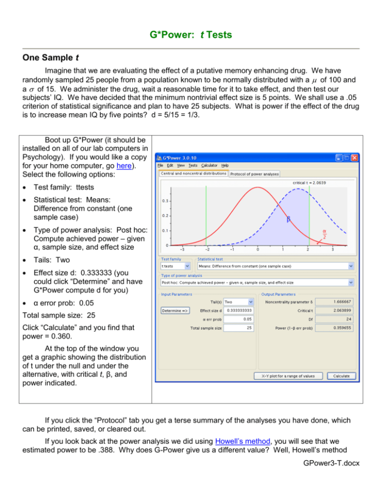
G*Power: t Tests
One Sample t
Imagine that we are evaluating the effect of a putative memory enhancing drug. We have
randomly sampled 25 people from a population known to be normally distributed with a  of 100 and
a  of 15. We administer the drug, wait a reasonable time for it to take effect, and then test our
subjects’ IQ. We have decided that the minimum nontrivial effect size is 5 points. We shall use a .05
criterion of statistical significance and plan to have 25 subjects. What is power if the effect of the drug
is to increase mean IQ by five points? d = 5/15 = 1/3.
Boot up G*Power (it should be
installed on all of our lab computers in
Psychology). If you would like a copy
for your home computer, go here).
Select the following options:

Test family: ttests

Statistical test: Means:
Difference from constant (one
sample case)

Type of power analysis: Post hoc:
Compute achieved power – given
α, sample size, and effect size

Tails: Two

Effect size d: 0.333333 (you
could click “Determine” and have
G*Power compute d for you)

α error prob: 0.05
Total sample size: 25
Click “Calculate” and you find that
power = 0.360.
At the top of the window you
get a graphic showing the distribution
of t under the null and under the
alternative, with critical t, β, and
power indicated.
If you click the “Protocol” tab you get a terse summary of the analyses you have done, which
can be printed, saved, or cleared out.
If you look back at the power analysis we did using Howell’s method, you will see that we
estimated power to be .388. Why does G-Power give us a different value? Well, Howell’s method
GPower3-T.docx
2
assumes that our sample size is large enough that the t distribution is well approximated by the
normal curve. With N = 25 the t distribution has fatter tails than the normal curve, and that lowers our
power a bit.
At the bottom of the window you can click “X-Y plot for a range of values.” Select what you
want plotted on Y and X and set constants and then click “Draw plot.” Here is the plot showing the
relation ship between sample size and power. Clicking the “Table” tab gives you same information in
a table.
We are unhappy with 36% power. How many subjects would we need to have 95% power?
Under Type of power analysis, select “A priori: Compute required sample size given α, power, and
effect size.” Enter “.95” for “Power (1- β err prob).” Click “Calculate.” G*Power tells you that you
need 119 subjects to get the desired power.
3
Independent Samples t
We wish to compare the Advanced Psychology GRE scores of students in general psychology
masters programs with that of those in clinical psychology masters programs. We decide that we will
be satisfied if we have enough data to have an 80% chance of detecting an effect of 1/3 of a standard
deviation, employing a .05 criterion of significance. How many scores do we need in each group, if
we have the same number of scores in each group?
Select the following options:

Test family: ttests

Statistical test: Means: Difference between two independent means (two groups)

Type of power analysis: A priori: Compute required sample size given α, power, and effect size

Tails: Two

Effect size d: 0.333333 (you could click “Determine” and have G*Power compute d for you)

α error prob: 0.05

Power (1- β err prob): .8

Allocation ratio N2/N1: 1
Click “Calculate” and you see that you need 143 cases in each group, that is, a total sample
size of 286.
Change the allocation ratio to 9 (nine times as many cases in the one group than in the other)
and click “Calculate” again. You will see that you would need 788 subjects to get the desired power
with such a lopsided allocation ratio.
Consider the following a posteriori power analysis. We have available only 36 scores from
students in clinical programs and 48 scores from students in general programs. What are our
chances of detecting a difference of 40 points (which is that actually observed at ECU in 1981) if we
use a .05 criterion of significance and the standard deviation is 98?
Change the type of power analysis to Post hoc. Enter d = 40/98 = .408, n1 = 36, n2 = 48. Click
“Calculate.” You will see that you have 45% power.
Output:
Noncentrality parameter δ
= 1.850514
Critical t
= 1.989319
Df
= 82
Power (1-β err prob)
= 0.447910
Correlated Samples t
I am testing the effect of a new drug on performance on a task that involves solving anagrams.
I want to have enough power to be able to detect an effect as small as 1/5 of a standard deviation (d
= .2) with 95% power – I consider Type I and Type II errors equally serious and am employing a .05
criterion of statistical significance, so I want beta to be not more than .05. I shall use a correlated
samples design (within subjects) and two conditions (tested under the influence of the drug and not
under the influence of the drug). In previous research I have found the correlation between
d
.2

 .3162 .
conditions to be approximately .8. d Diff 
2(1  12 )
2(1  .8)
4
Use the following settings:

Statistical test: Means: Difference between two dependent means (matched pairs)

Type of power analysis: A priori: Compute required sample size given α, power, and effect size

Tail(s): Two

Effect size dz: .3162

α error prob: 0.05

Power (1- β err prob): .95
Click “Calculate.” You will find that you need 132 pairs of scores.
Output:
Noncentrality parameter δ
= 3.632861
Critical t
= 1.978239
Df
= 131
Total sample size
= 132
Actual power
= 0.950132
Consider the following a posteriori power
analysis. We assume that GRE Verbal and GRE
Quantitative scores are measured on the same
metric, and we wish to determine whether
persons intending to major in experimental or
developmental psychology are equally skilled in
things verbal and things quantitative. If we
employ a .05 criterion of significance, and if the
true size of the effect is 20 GRE points (that was
the actual population difference the last time I
checked it, with quantitative > verbal), what are
our chances of obtaining significant results if we
have data on 400 persons? We shall assume
that the correlation between verbal and
quantitative GRE is .60 (that is what it was for
social science majors the last time I checked).
We need to know what the standard deviation is
for the “dependent variable,” GRE score. The
last time I checked, it was 108 for verbal, 114 for
quantitative.
Change type of power analysis to “Post hoc.” Set the total sample size to 400. Click on
“Determine.” Select “from group parameters.” Set the group means to 0 and 20 (or any other two
means that differ by 20), the standard deviations to 108 and 114, and the correlation between groups
to .6. Click “Calculate” in this window to obtain the effect size dz, .2100539.
Click “Calculate and transfer to main window” to move the effect size dz to the main window.
Click “Calculate” in the main window to compute the power. You will see that you have 98% power.
5
Pearson r
Consider the following a priori power analysis. We wish to determine whether or not there is a
correlation between misanthropy and support for animal rights. We shall measure these attributes
with instruments that produce scores for which it is reasonable to treat the variables as continuous.
How many respondents would we need to have a 95% probability of obtaining significant results if we
employed a .05 criterion of significance and if the true value of the correlation (in the population) was
0.2?
Select the following options:

Test family: ttests

Statistical test: Correlation: Point biserial model (that is, a regression analysis)

Type of power analysis: A priori: Compute required sample size given α, power, and effect size

Tails: Two

Effect size |r|: .2

α error prob: 0.05

Power (1- β err prob): .95
Click “Calculate” and you will see that you need 314 cases.
t tests - Correlation: Point biserial model
Analysis:
A priori: Compute required sample size
Input:
Tail(s)
= Two
Effect size |r|
= .2
α err prob
= 0.05
Power (1-β err prob)
= 0.95
Noncentrality parameter δ
= 3.617089
Critical t
= 1.967596
Df
= 312
Total sample size
= 314
Actual power
= 0.950115
Output:
6
Check out Steiger and Fouladi’s R2 program, which will do power analysis (and more) for
correlation models, including multiple correlation.
Install GPower on Your Personal Computer
If you would like to install GPower on your Windows computer, you can download it from
Universität Duesseldorf.
Return to Wuensch’s Statistics Lessons Page
January, 2014.