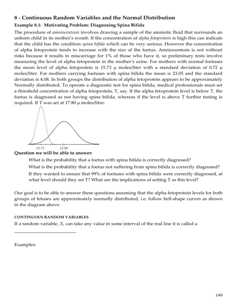
8 - Continuous Random Variables and the Normal Distribution
Example 8.1: Motivating Problem: Diagnosing Spina Bifida
The procedure of amniocentesis involves drawing a sample of the amniotic fluid that surrounds an
unborn child in its mother’s womb. If the concentration of alpha fetoprotein is high this can indicate
that the child has the condition spina bifida which can be very serious. However the concentration
of alpha fetoprotein tends to increase with the size of the foetus. Amniocentesis is not without
risks because it results in miscarriage for 1% of those who have it, so preliminary tests involve
measuring the level of alpha fetoprotein in the mother’s urine. For mothers with normal foetuses
the mean level of alpha fetoprotein is 15.73  moles/liter with a standard deviation of 0.72 
moles/liter. For mothers carrying foetuses with spina bifida the mean is 23.05 and the standard
deviation is 4.08. In both groups the distribution of alpha fetoprotein appears to be approximately
Normally distributed. To operate a diagnostic test for spina bifida, medical professionals must set
a threshold concentration of alpha fetoprotein, T, say. If the alpha fetoprotein level is below T, the
foetus is diagnosed as not having spina bifida, whereas if the level is above T further testing is
required. If T was set at 17.80  moles/litre:
15.73
23.05
Question we will be able to answer:
What is the probability that a foetus with spina bifida is correctly diagnosed?
What is the probability that a foetus not suffering from spina bifida is correctly diagnosed?
If they wanted to ensure that 99% of foetuses with spina bifida were correctly diagnosed, at
what level should they set T? What are the implications of setting T as this level?
Our goal is to be able to answer these questions assuming that the alpha fetoprotein levels for both
groups of fetuses are approximately normally distributed, i.e. follow bell-shape curves as shown
in the diagram above.
CONTINUOUS RANDOM VARIABLES
If a random variable, X, can take any value in some interval of the real line it is called a
__________________________
Examples:
149
STAT 305: Chapter 8 – Continuous Random Variables and the Normal Distribution
Fall 2013
THE STANDARDIZED HISTOGRAM or DENSITY SCALING
Example 8.2: Dietary Carbohydrate: The average daily intake of carbohydrate (g/day) in the diet
found for a sample n=5929 people.
The histogram of the data given in Graph (a) shows the carbohydrate intake. From this we see
that:
*
*
*
(b ) A re a b e tw e e n a = 2 2 5
an d b = 3 7 5 sh ad ed
( a ) S ta n d a r d iz e d h is to g ra m
S h a d e d a re a = .4 8 3
.0 0 4
.0 0 4
.0 0 2
.0 0 2
.0 0 0
0
200
400
600
( c ) WC iatrb
h oahpypdrra
o xtei m a(gt i/d
n ag y c) u r v e
.0 0 4
.0 0 0
800
(C o rre s p o n d s to 4 8 .3 %
o f o b s e rv a tio n s )
0
600
37e5e n a = 2 2 5
( d ) A r2e2a5 b e t w
an d b = 3 7 5 sh ad ed
S h a d e d a re a = .4 8 6
.004
.002
800
(c f. a re a = .4 8 3
f o r h is to g r a m )
.002
0
200
400
C a r b o h y d r a te
600
( g/d a y )
800
0
600
225
800
375
Note: Histograms are usually drawn with the height of the rectangle for the ith interval being the frequency,
(representing the count) or the relative frequency (representing the proportion).
The standardized histogram adjusts the height of the rectangle to ____________________
__________________________________________________.
i.e. The area of the ith rectangle tells us what proportion of the data lie in the ith class interval.
For a standardized histogram:
The vertical scale is : Relative frequency/interval width  this is called the density scale.
Total area under the histogram = ______
The proportion of the data between a and b is __________________________________________
Carbohydrate Example (cont’d)
The proportion of people with carbohydrate intakes between 225 and 375 g/day is the shaded area in the
histogram in Graph (b) (= 0.483 or 48.3%)
Graph (c) shows an approximating smooth curve on the standardized histogram and on Graph (d) the area
from 225 to 375 is shaded. This area is calculated to be 0.486 and is very close to the actual proportion of
people who had carbohydrate intakes of between 225 and 375 g/day.
150
Example 8.3: Cell Radii of Malignant Breast Tumors (see Assignment #2)
In JMP we can add a density scale axis to a histogram in JMP select Histogram Options > Density
Axis.
The histogram on the left is for cell radii of malignant tumor cells
from the fine needle aspirations in the breast cancer study on your
second assignment. Here the class intervals all have width 1 so the
area of any bar is simply the density axis value, hence the heights of
the bars here represent empirical probabilities. For example if we let
X = radius of a randomly selected malignant tumor cell
we estimate that the P(14 < X < 15)  .10 or a10% chance.
Example 8.4: Spina Bifida (SpinaBifida.JMP)
To obtain a standardized histogram in JMP select Histogram Options > Density Axis. This is a histogram of
the alpha fetoprotein levels of women who are carrying a foetus with spina bifida.
The shaded area in the histogram above is 2.5 (width of the interval) times .10 (height of the bar in the
standardized scale) which is .25. This says that the estimated probability that the alpha fetoprotein level
found in the urine of a mother carrying a foetus with spina bifida lies between 22.5  moles/liter and 25 
moles/liter is .25, or a 25% chance.
If we define X = alpha fetoprotein level found in the urine of mothers carrying a foetus with spina bifida
we can say the following:
P(22.5  X  25)  .25 or 25% chance
Note: Examination of the spreadsheet confirms that the number of observations highlighted is exactly 25 of the 100 observations.
151
STAT 305: Chapter 8 – Continuous Random Variables and the Normal Distribution
Fall 2013
DENSITY/SMOOTH CURVES
Take a standardized histogram, decrease the width of the class intervals and increase the number
of observations. Then the top of the histogram tends to a smooth curve.
n = 500
n = 100
n = 10000
n =100000
n = 1,000,000
0.08
0.05
Density
0.10
0.03
10
20
30
40
The limiting smooth curve can be described using a function called the probability density
function.
To obtain a sampled-based estimate of this function in JMP select Analyze > Distribution > Fit
Distribution > Smooth Curve. As n increases, as shown above the histogram itself “converges” to
the probability density function.
PROPERTIES OF THE PROBABILITY DENSITY FUNCTION (p.d.f.),
1.
f(x)
(i.e. the p.d.f. curve stays above the x-axis)
2.
Pa  X  b =
3.
Area under the p.d.f. curve =
ENDPOINTS OF INTERVALS
For a continuous random variable, X, endpoints of intervals are ___________________
Pa  X  b =
152
(Inclusion or exclusion of the endpoints will not change the area.)
THE NORMAL DISTRIBUTION
Examples: Alpha fetoprotein levels of mothers carrying a foetus with spina bifida.
Limiting distribution that is a smooth bell shaped symmetric curve is
called the Normal p.d.f. curve or just the Normal curve.
50% 50%
Mean
If a random variable, X, has a Normal distribution with a mean  and a standard deviation  we write:
The Normal distribution is important because:

it fits a lot of data reasonably well;

it can be used to approximate other distributions (e.g. binomial)

it is important in statistical inference (see later inferential methods in the course.)
Shape is solely determined by  and  , the population mean  controls where the normal is centered, and
the population standard deviation  controls the spread about  .
Example: Alpha fetoprotein levels found in the urine of mothers carrying a foetus with spina bifida.
Let X = alpha fetoprotein level in the urine of a mother carrying a foetus with spina bifida.
The mean AFP level is _________  moles/liter and the standard deviation is __________  moles/liter.
EMPIRICAL RULE
Approximately _______ % of the mothers in this population will have AFP levels within 1 standard
deviation of the mean, i.e. we estimate that approximately ________% of this population of mothers will
have AFP levels:
between _______________ and ________________
= between _______________ and ________________
.
Approximately _______ % of the mothers in this population will have AFP levels within 2 standard
deviation of the mean, i.e. we estimate that approximately ________% of this population of mothers will
have AFP levels:
between _____________ and ______________
= between _____________ and ______________
Approximately _______ % of the mothers in this population will have AFP levels within 3 standard
deviation of the mean, i.e. we estimate that approximately ________% of this population of mothers will
have AFP levels:
between _____________ and ________________
= between ______________ and ________________
153
STAT 305: Chapter 8 – Continuous Random Variables and the Normal Distribution
Fall 2013
For the Normal Distribution:
68% chance of falling within 1  of  ;
95% chance of falling within 2  of  ;
99.7% chance of falling within 3  of  .
A random observation has approximately:
or
68% of observations are within 1  of  ;
95% of observations are within 2  of  ;
99.7% of observations are within 3  of  .
In a Normal distribution, approximately:
OBTAINING OTHER PROBABILITES ASSOCIATED WITH A NORMAL DISTRIBUTION
Normal distribution probabilities can be obtained from all statistical packages by giving the mean and
standard deviation of the distribution. (see Normal Probability Calculator in Tutorials section of website)
Most table and computer packages calculate the value of P(X  x). i.e. cumulative or lower tail probabilities.
Area = P(X  x)
OR
Area = P(X  x)
x
Standardization and the Standard Normal Distribution
Fact:
If X ~ N(  ,  ) then if we define a new random variable Z 
x
X 
then Z ~ N(0,1)

i.e. we create a new random variable Z where the observed values of Z are the z-scores for the random
variable X. The process of converting a random variable X to z-scores is called standardization.
Basic method for obtaining probabilities
1.
Sketch a Normal curve, marking the mean and the value(s) of interest.
2.
Shade the area under the curve corresponding to the required probability.
3.
Convert all values in original scale to their corresponding z-scores.
4.
Obtain the desired probability from the lower-tail areas provided by the standard normal table found
in the front inside cover of the text.
154
Find the following standard normal probabilities using the Standard Normal Table
a) P(Z < .67)
b) P(Z > 2.25)
c) P(Z > 3.00)
e) P(Z < -2.33)
f) P(-1.96 < Z < 1.96)
h) Find z so that P(Z < z) = .90, i.e. what is the 90th percentile of the standard normal distribution?
Example 8.1 : Spina Bifida Example (continued)
X = AFP level of a randomly selected mother carrying a foetus with spina bifida . Lets assume that
X~Normal ( =23.05,  = 4.08) using the sample mean and sample standard deviation.
Find the following:
a) P(X < 15.00)
=
155
STAT 305: Chapter 8 – Continuous Random Variables and the Normal Distribution
Fall 2013
b) P(X < 27.00)
c) P(X > 17.0)
d) Find the 90th percentile.
e) Find the 25th percentile
Example 8.1: Spina bifida original questions
15.73
23.05
Recall: For normal fetuses  =15.73,  = 0.72 and for foetuses with spina bifida  = 23.05 and  = 4.08.
Assume the threshold for detecting spina bifida is set at 17.8. (A fetus would be diagnosed as not having
spina bifida if the fetoprotein level is below 17.8)
a)
What is the probability that a fetus not suffering from spina bifida is correctly diagnosed?
b)
What is the probability that a fetus with spina bifida is correctly diagnosed?
156
c)
d)
If they wanted to ensure that 99% of foetuses with spina bifida were correctly diagnosed, at what level
should they set T ?
What would be the consequences of using this value for the threshold (T)?
157
STAT 305: Chapter 8 – Continuous Random Variables and the Normal Distribution
Fall 2013
Standard Normal Table – P(Z < z)
Table for negative z-scores, i.e. z < 0
158
Standard Normal Table – P(Z < z)
Table for positive z-scores, i.e. z > 0
159