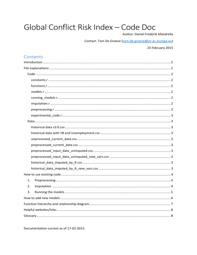
Global Conflict Risk Index – Code Doc
Author: Daniel Frederik Mandrella
Contact: Tom De Groeve (tom.de-groeve@jrc.ec.europa.eu)
23 February 2015
Contents
Introduction ............................................................................................................................................ 2
File explanations ..................................................................................................................................... 2
Code .................................................................................................................................................... 2
constants.r ...................................................................................................................................... 2
functions.r ....................................................................................................................................... 2
models.r .......................................................................................................................................... 2
running_models.r ............................................................................................................................ 2
imputation.r .................................................................................................................................... 2
preprocessing.r ............................................................................................................................... 3
experimental_code.r ....................................................................................................................... 3
Data ..................................................................................................................................................... 3
historical data v3.0.csv .................................................................................................................... 3
historical data with YB and Unemployment.csv ............................................................................. 3
unprocessed_current_data.csv....................................................................................................... 3
preprocessed_current_data.csv ..................................................................................................... 3
preprocessed_input_data_unimputed.csv ..................................................................................... 3
preprocessed_input_data_unimputed_new_vars.csv ................................................................... 3
historical_data_imputed_by_R.csv ................................................................................................. 3
historical_data_imputed_by_R_new_vars.csv ............................................................................... 3
How to use existing code ........................................................................................................................ 4
1.
Preprocessing .............................................................................................................................. 4
2.
Imputation .................................................................................................................................. 4
3.
Running the models .................................................................................................................... 5
How to add new models ......................................................................................................................... 6
Function hierarchy and relationship diagram ......................................................................................... 7
Helpful websites/links ............................................................................................................................. 8
Glossary ................................................................................................................................................... 8
Documentation current as of 17-02-2015.
Introduction
The purpose of this documentation is to explain the structure and purpose of the existing code and
related tools for the Global Conflict Risk index (GCRI), how to modify, and how to add to it. As the code
is work-in-progress, so is this documentation, and the two might diverge at some points. Critical
evaluation is always required in such cases in order to find out which of the two (the code, or the
documentation) is wrong/outdated.
The next section of this documentation will briefly explain what code is in which files, and what to do
with it. Then, an explanation will be provided about how to use the existing code to run models, apply
them, what to look out for, and so on. Then, a run-down of how to modify it, e.g. to add new models,
and what modifications are necessary in which places, will be given. Lastly, a collection of helpful links
and websites can be found in the subsequent section. This is mostly for looking for answers for
technical or statistical questions, as well as general explanations of approaches used so far. The final
section is a brief glossary to explain some of the vocabulary used in the code, variable names, code
comments, etc.
The current iteration and most updated version of the code can be found in the folder:
G:\PROJECTS_CRITECH\DG_2014_EEAS_CONFLICTRISKINDEX\METHODOLOGY\MODEL\MODEL 2015 FEBRUARY
(IGNORE FOR NOW -- DANIEL)
File explanations
Code
constants.r
This file just contains all constant variables that are used throughout the other code files. This is also
where the kClassifierThreshold variable can be found and changed if needed.
functions.r
This file contains all R-functions for running the models, applying them to both historical and most
recent data, etc. It does not execute any code and is just a “repository” of sorts for all functions (except
the models) that are used throughout the other files. If you find any kind of function anywhere that is
not a statistical model, look for it in this file. For more details on each function, see directly in their
definitions in the file. Every function is extensively commented with expected inputs, outputs, general
descriptions of their functionalities, etc.
models.r
This file contains all statistical models. Every model is realized as a function, and every function/model
basically executes the same steps, and accepts the same arguments. For a more detailed explanation
of the arguments, see in the file directly.
running_models.r
This is the central file that contains the scripts to actually use the functions from functions.r and
models from models.r. If any kind of output other than imputation or preprocessing are to be run,
then do it with the code from this file.
imputation.r
This file contains the scripts to impute all data sets with missing variables, i.e. the historical dataset.
The functions to do this are in functions.r, so this file only sources and executes them, and additionally
does some data munging/arranging. Imputation is done AFTER preprocessing (see below).
preprocessing.r
File containing the scripts to do various smaller preprocessing tasks, including computing whether any
given country-year is a ‘peace’, ‘war’, or ‘onset’ year. Also adds a new column containing the country’s
region according to EEAS classification. This is needed for the models incorporating region as a random
factor.
experimental_code.r
As the name suggest. Some first tries at Bayesian regression analysis and related. Not used to produce
any kind of output.
Data
historical data v3.0.csv
As the name suggests, this is the csv file holding the historical data from 1989 to 2009 for all
independent variables, conflict data, and country-years. It does not include war/peace/onset columns,
and uses the more verbose column names (i.e. GCRI.POL.REG_P2 vs. non-verbose REG_P2). This file is
read in by preprocessing.r for preprocessing purposes.
historical data with YB and Unemployment.csv
This data set is identical to “historical data v3.0.csv” except that it also includes a few new independent
variables, notably CORRUPT, YOUTHBMALE, YOUTHBBOTH, and INEQ_SWIID. YOUTHBMALE and
YOUTHBOTH respectively refer to youth bulge calculated for only males, and for both genders.
unprocessed_current_data.csv
This is the csv file containing the most recent/current data, e.g. only the data for all countries in 2014.
It is supposed to be used to apply the models and come up with predictions.
preprocessed_current_data.csv
As the name suggests, this is the preprocessed version of the above.
preprocessed_input_data_unimputed.csv
This is the historical data without the new variables after it has gone through preprocessing, but before
it has been imputed.
preprocessed_input_data_unimputed_new_vars.csv
This is the historical data with new variables after it has gone through preprocessing, but before it has
been imputed.
historical_data_imputed_by_R.csv
This is the historical data without new variables after it has gone through both preprocessing and
imputation. It is now ready to be used for running the models.
historical_data_imputed_by_R_new_vars.csv
This is the historical data with new variables after it has gone through both preprocessing and
imputation. It is now ready to be used for running the models.
How to use existing code
Data processing workflow
2. imputation.r
1. preprocessing.r
3. running_models.r
source()
source()
source()
functions.r
models.r
constants.r
1. Preprocessing
The first step is the preprocess the data sets. The current iteration of the preprocessing script does
the following:
-
-
It reads in the historical data
It orders historical data first by ISO code, then by year, such that:
o AFG 2009
o AFG 2008
o …
o ZWE 1990
o ZWE 1989
It then calculates Boolean vectors for single-year Violent and Highly Violent conflicts, for each
conflict dimension; it attaches these new vectors as columns to the historical data set
It then switches the column names from verbose to less verbose (i.e. from GCRI.POL.REG_P2
to just REG_P2), computes whether a given country-year is in ‘war’, ‘peace’, or ‘onset’ for
every conflict dimension and intensity level (i.e. four new columns), and it adds a new column
denoting every country’s region according to EEAS classification
Note that the script does this twice currently: once for the data set without the new variables (YOUTHB
and UNEMP at the moment) and once for the data set that includes those. The script also preprocesses
the most recent data by switching column names and converting the relevant columns to numeric.
2. Imputation
The imputation script first loads the preprocessed data in (pay attention that the name of the output
file from preprocessing.r matches the name of the input file name in imputation.r). It splits the data
into several data frames because only the main variables need to be imputed, and the other ones
should not be used to impute those. The MICE (Multiple Imputation by Chained Equations) package
then imputes the data 10 times with the mice() function. The complete() function then creates a
complete data set by combining one of the imputations with the original existing data (these
imputations are the variables d0, d1, d2, …, etc.). The imputations are then simply averaged, the full
data set is reconstructed (this is the reversal of splitting the data in the beginning), and saved to a new
csv file.
Similarly to the preprocessing.r script, the imputation is done twice, once for the data set without the
new variables, and once for the data set with them. Execute the one needed, they are both
independent of each other, including loading the required packages, setting the random number
generator seed, etc.
3. Running the models
The running_models.r script is the centrepiece of the code base from which all of the actual execution
of models is done. The file is partitioned into a few different sections. The first one called “Setup”
loads required packages, sources the functions.r, models.r, and constants.r files, and sets the seed for
the random number generator. It also sets the working directory: this needs to be changed according
to where the other files actually are. If the next iteration of the overall model is for example Model
2015 March, then the path needs to be changed accordingly. Otherwise it might accidentally execute
models and code from a previous iteration.
Running one or more models works like this:
-
-
-
-
-
-
A list object simply called “models” should contain named (!) elements corresponding to the
model functions from models.r that should be run, i.e. an element called BaseModel(), an
element called AllInteractions(), etc.
Model functions can be added to the “models” list simply via assigning them like this:
o models[[‘ModelName’]] <- ModelName
o ModelName has to be a model function specified in models.r
The string in the double brackets is the name the element in the list is given, and the list can
be indexed by these names (in other programming languages, e.g. Python, this is akin to a
dictionary where the keys are strings and the values are functions)
The named list of models is then passed to the runModels() function, along with the data with
which the models should be trained and evaluated
o A variety of additional arguments can be passed to runModels(), including the
threshold, if cross validation should be used, etc. – see the function specification in
functions.r for more details)
o Note that the data passed to runModels() should be the historical data; this function
is only supposed to run a variety of models and compare their performance – if the
models should be applied, see the applyModels() function instead
Since the output of the runModels() is difficult to read if a lot of models have been run, the
function compareModels() summarizes the results in a comparison matrix where the different
metrics are in the columns and the model names in the rows; this function also allows to save
this comparison matrix in a .csv file
The compareModels() function also includes the possibility to pass an additional string via the
custom.name argument that will be added to the file name in case the matrix is saved to csv.
This is useful if the same models are run with different thresholds, with or without cross
validation, etc., so that in the end the different comparison matrices do not override each
other
Applying the models to the most recent data works similarly to running the models to compare
performances. The list of models that should be applied is passed to the applyModels() function, along
with the training data (“train.data” argument) and the most recent data (“apply.data” argument).
Additional arguments exist, see the function specification for details. Note that the applyModels()
function does not depend on having previously executed the models via runModels() or similar.
Instead, it runs the models on the training data (without cross validation), and then predicts new
intensity values for the most recent data via predict().
The reasoning behind this setup is as follows: with the runModels() function, the best model in terms
of performance can be found. Preferably, this is done via cross validation to reduce the risk of
overfitting when using the whole data set for training and testing. If it is done via cross validation, in
each iteration (i.e. for each fold), only a subset of the data is used to calculate the coefficients.
However, when applying the model to the most recent data, all the data should be used to train the
model since this choice of parameters (the variables) and statistical model (logistic, zero-inflated
negative binomial, etc.) has been found to perform best with cross validation. So instead of using a
subset of the historical data, all historical data is used in applyModels().
The output from applyModels() is a named list where each element consists of the most recent data
plus six columns representing that specific model’s predicted probabilities, intensities, and overall
predictions for both the national power and subnational conflict dimensions. Using the
saveAppliedModelsOutput() function, these lists can be saved to .csv files where the file name
corresponds to the respective model. As an example, if applyModels() produces a named list of length
2 where the first element is the most recent data plus the forecasts from BaseModel, and the second
element the same with the forecasts from AllInteractions, then saveAppliedModelsOutput() will
produce two output csv files named “2015-02-12__AllInteractions__applied-to-historical.csv” and
“2015-02-12__BaseModel__applied-to-historical.csv” (note: “applied to historical” refers to the fact
that the output is the historical data set with predictions from the model for the historical data; the
other option is “applied-to-most-recent” indicating the forecasts for the most recent data). The results
can then further be analysed and visualised in Excel.
How to add new models
In order to add new models to the existing infrastructure, three things have to be done.
1. In the models.r file, a function has to be added that executes the statistical model(s),
calculates their performance metrics, and creates the predictions from the model. The overall
structure of this function is the same for all statistical models, and most of the code can be
copied from existing ones. Based on the input for the conflict.dimension argument, the
function should be usable for both national power and subnational predictions. For this
reason, the dependent variables for these two types should not be hardcoded into the model
specifications but instead be assigned depending on the input. The formula for the model
specification is currently created by the combination of the paste() and as.formula() functions.
See ?paste and ?as.formula for more information on how these work. Overall, keep as close
to the structure of existing model functions.
2. When the new model function has been specified, a new function to calculate the predictions
for this new model has to be written in the functions.r file. Currently existing prediction
functions are for example computePredictionsGLMandLM() for the combination of a
generalized linear model (logistic model) with a standard linear model; another is
computePredictionsZEROINFLorHURDLE(), for zero-inflated negative binomial and hurdle
models respectively. These functions are usually just wrappers around predict() functions with
a few auxiliary tasks added (e.g. limiting the predictions to a maximum of 10 or minimum of
0), and in the case of two combined models, the combination of the two via a static or dynamic
threshold (e.g. if the first is a logistic model predicting probabilities, and the second is a linear
model predicting intensities, then the combination of the two means to assign a final
prediction value equal to the predicted intensity if and only if the predicted probability for
that country-year is above a certain threshold – and zero otherwise).
3. When the above two functions have been written, the last thing to do, is to modify the
computePredictions() function to call the appropriate sub-functions for the particular types of
models passed to computePredictions(). To illustrate, computePredictions() checks the
classes/types of the statistical models passed to it, and if those are for example ‘glm’ and ‘lm’,
it calls computePredictionsGLMandLM(); if the first model instead is ‘zeroinfl’ and the second
model is ‘NULL’ (i.e. there was none), then it calls computePredictionsZEROINFLorHURDLE();
etc.
See the graphic on the next page for a visual illustration of function hierarchy.
Function hierarchy and relationship diagram
ModelFunction()
6. results
1. call
3. input
calculateMetrics()
5. results
4. call
determineOutcome()
computePredictions()
2. call
(example functions)
computePredictionsTwoLasso()
computePredictionsZEROINFLorHURDLE()
computePredictionsGLMandLM()
2.5 call if
threshold == ‘dynamic’
determineThresholdDynamically()
Helpful websites/links
For a code style guide, I have mostly followed Google’s R Style Guide found here: https://googlestyleguide.googlecode.com/svn/trunk/Rguide.xml
I did make some modifications, however. For example, instead of using UpperCamelCase I used
LowerCamelCase, and the model functions are not named according to the guide.
For statistics-related questions, Cross Validated (http://stats.stackexchange.com/) is a great resource.
For programming-related problems, Stack Overflow (http://stackoverflow.com/) is the go-to address.
Glossary