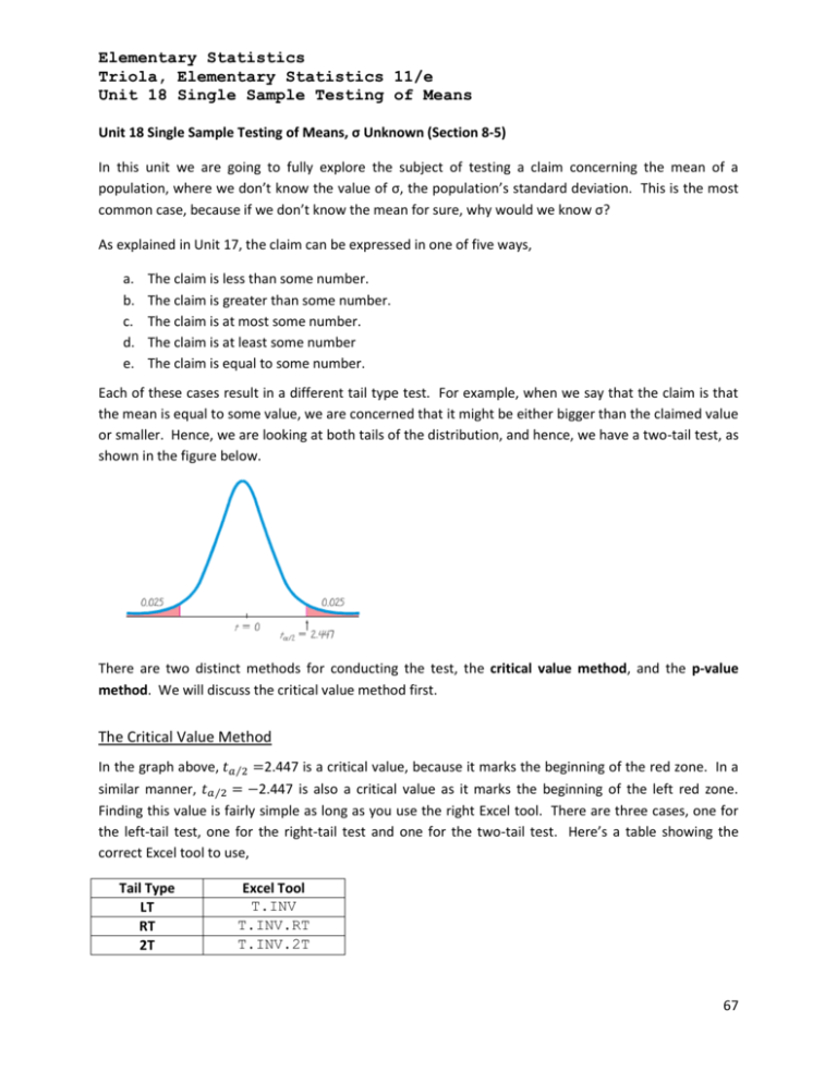
Elementary Statistics
Triola, Elementary Statistics 11/e
Unit 18 Single Sample Testing of Means
Unit 18 Single Sample Testing of Means, σ Unknown (Section 8-5)
In this unit we are going to fully explore the subject of testing a claim concerning the mean of a
population, where we don’t know the value of σ, the population’s standard deviation. This is the most
common case, because if we don’t know the mean for sure, why would we know σ?
As explained in Unit 17, the claim can be expressed in one of five ways,
a.
b.
c.
d.
e.
The claim is less than some number.
The claim is greater than some number.
The claim is at most some number.
The claim is at least some number
The claim is equal to some number.
Each of these cases result in a different tail type test. For example, when we say that the claim is that
the mean is equal to some value, we are concerned that it might be either bigger than the claimed value
or smaller. Hence, we are looking at both tails of the distribution, and hence, we have a two-tail test, as
shown in the figure below.
There are two distinct methods for conducting the test, the critical value method, and the p-value
method. We will discuss the critical value method first.
The Critical Value Method
In the graph above, 𝑡𝑎⁄2 =2.447 is a critical value, because it marks the beginning of the red zone. In a
similar manner, 𝑡𝑎⁄2 = −2.447 is also a critical value as it marks the beginning of the left red zone.
Finding this value is fairly simple as long as you use the right Excel tool. There are three cases, one for
the left-tail test, one for the right-tail test and one for the two-tail test. Here’s a table showing the
correct Excel tool to use,
Tail Type
LT
RT
2T
Excel Tool
T.INV
T.INV.RT
T.INV.2T
67
Elementary Statistics
Triola, Elementary Statistics 11/e
Unit 18 Single Sample Testing of Means
Here are three examples showing how each tool is used.
Case 1 LT Test
𝐻0 : 𝜇 = 𝑠𝑜𝑚𝑒 𝑐𝑙𝑎𝑖𝑚
𝐻1 : 𝜇 < 𝑠𝑜𝑚𝑒 𝑐𝑙𝑎𝑖𝑚
𝑥̅ = 25.08
𝑠 = .875
𝑛 = 30
𝐶. 𝐿. = 95% (𝛼 = 0.05)
𝑡𝑎⁄2 = T. INV(α, df) = T. INV(0.05, 29) = −1.6991
Notice that the critical value is negative, which makes perfectly good sense since we’re concerned about
ending up in the left red zone. Now, let’s take a look at a right tail test.
Case 2 RT Test
𝐻0 : 𝜇 = 𝑠𝑜𝑚𝑒 𝑐𝑙𝑎𝑖𝑚
𝐻1 : 𝜇 > 𝑠𝑜𝑚𝑒 𝑐𝑙𝑎𝑖𝑚
𝑥̅ = 25.08
𝑠 = .875
𝑛 = 30
𝐶. 𝐿. = 95% (𝛼 = 0.05)
There’s one huge wrinkle and it’s because Microsoft is a crap company. There is no T.INV.RT! What to
do? Well, we can use T.INV, but instead of using 𝛼 for the probability, we use 1 − 𝛼. Hence,
𝑡𝑎⁄2 = T. INV. RT(1 − α, df) = T. INV. RT(0.95, 29) = 1.6991
Note that the critical value is the same number as for Case 1, but now it’s positive. Since the Student-t
distribution is symmetrical this should come as no big surprise.
Finally, we deal with the two-tail case.
Case 1 2T Test
𝐻0 : 𝜇 = 𝑠𝑜𝑚𝑒 𝑐𝑙𝑎𝑖𝑚
𝐻1 : 𝜇 ≠ 𝑠𝑜𝑚𝑒 𝑐𝑙𝑎𝑖𝑚
𝑥̅ = 25.08
𝑠 = .875
𝑛 = 30
𝐶. 𝐿. = 95% (𝛼 = 0.05)
𝑡𝑎⁄2 = T. INV. 2T(α, df) = T. INV. 2T(0.05, 29) = 2.0452
Ok, now that we’ve got the critical values, what do we do with them? Well, we want to know if our
calculated t-score (see the previous unit) lies in the red zone, and we do that by comparing our t-score
to the critical value. Again, we have to consider the tail type test we’re doing. First, we calculate our tscore,
𝑡=
𝑥̅ − 𝜇
√𝑛
𝑠
where the value of 𝜇 is the claim
68
Elementary Statistics
Triola, Elementary Statistics 11/e
Unit 18 Single Sample Testing of Means
Then we do the following comparisons,
Left Tail
If the t-score < critical value (they both would be negative numbers) then the t-score is going to
be in the left red zone and we would reject the null hypothesis. Otherwise, we fail to reject the
null hypothesis.
Right Tail
If the t-score > critical value then the t-score is in the right red zone and we would reject the null
hypothesis. Otherwise, we fail to reject the null hypothesis.
Two Tail
If the absolute value of the t-score < critical value, we reject the null hypothesis. Remember to
first take the absolute value of the t-score before comparing it to the two-tail critical value. You
do this just for the two-tail test. Otherwise, we fail to reject the null hypothesis.
The p-Value Method
The p-Value Method works by comparing areas under the curve. In a single tail test and given that the
confidence level is 95%, the area under the tail is 0.05, which is the value of 𝛼, the significance. If we
found the area to the right (RT test) or left (LT test) of our calculated t score, and that area was less than
𝛼, then the t-score would have to be in the red zone. Look at the graph at the top and think about it.
This area that is to the right or left of our t is called the p-Value. The rule for rejecting the null
hypothesis is very simple, because there is only one rule, regardless of the type of tail test.
If p-Value < 𝛼, then reject the null hypothesis, otherwise, fail to reject it.
We find the p-Value with Excel. t is the calculated t score and df are the degrees of freedom:
Left Tail Test
p-Value = T.DIST(t, df)
Right Tail Test
p-Value = T.DIST.RT(t, df)
Two Tail Test
p-Vale = T.DIST.2T(|𝑡|, df)
Notice the absolute value brackets around t. That’s because T.DIST.2T only works
with positive values, even though a negative t would be a valid value; another ‘gift’
from Microsoft.
69
Elementary Statistics
Triola, Elementary Statistics 11/e
Unit 18 Single Sample Testing of Means
Worked Example
Let’s say that we work for the4 Coca-Cola Company, and it’s our job to verify that, on average, the cans
of coke going out the door contain 12 oz. This is a two-tail test because, on one hand we don’t want the
cans to contain less than 12 oz because then we can be accused of false labeling. On the other hand, we
don’t want them to contain more than 12 oz, because, while nobody is likely to complain, we would be
giving product away for nothing.
We collect a simple random sample of 20 cans and calculate the following statistics,
𝑥̅ = 11.98 𝑠 = .76 𝑛 = 20
We’ll use a 95% confidence level for our test.
Hypotheses Statement
𝐻0 : 𝜇 = 12.00
𝐻1 : 𝜇 ≠ 12.00
Calculated t score
𝑡=
𝑥̅ − 𝜇
11.96 − 12.00
√20 = 0.1177
√𝑛 =
𝑠
0.76
Critical Value and p-Value
Here’s a spreadsheet for calculating both the critical value and the p-Value. Click on the values for t, t
critical value and pValue to see how these were calculated. Note that we are using the absolute value
when calculating the t score because this is a two-tail test.
x
11.98
s
n
0.76
20
claim
t
12 0.117688
CL
t crit val p-Value
0.95 2.093024 0.90755
Here’s a subtle point concerning the p-Value of a two tail test. The p-Value is the sum of the areas
under both tails. This is the value we compare to 𝛼 which is also the sum of the two red zones.
Result
Critical Value Method
𝑡 < 𝑡𝑎⁄2 (the critical value), therefore fail to reject the Null Hypothesis.
p-Value Method
p-Value < 𝛼, therefore fail to reject the Null Hypothesis
Conclusion
On the basis of our evidence, we cannot reject the claim that the cans of Coke contain, on average,
12 oz of Coca-Cola.
If you look under Miscellaneous on the website, Hypotheses Testing Chart SSM is a wonderful
summary of this Unit.
This is the end of Unit 18. In class, you will get more practice with these concepts
by working exercises in MyMathLab.
70