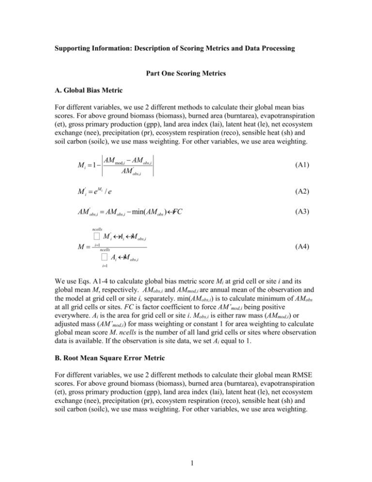
Supporting Information: Description of Scoring Metrics and Data Processing
Part One Scoring Metrics
A. Global Bias Metric
For different variables, we use 2 different methods to calculate their global mean bias
scores. For above ground biomass (biomass), burned area (burntarea), evapotranspiration
(et), gross primary production (gpp), land area index (lai), latent heat (le), net ecosystem
exchange (nee), precipitation (pr), ecosystem respiration (reco), sensible heat (sh) and
soil carbon (soilc), we use mass weighting. For other variables, we use area weighting.
AM mod,i - AM obs,i
'
AM obs,i
M i =1-
(A1)
M 'i = eMi / e
(A2)
AM 'obs,i = AM obs,i - min(AM obs )´ FC
(A3)
ncells
M=
åM
'
i
´ Ai ´ M obs,i
i=1
ncells
å A ´M
i
(A4)
obs,i
i=1
We use Eqs. A1-4 to calculate global bias metric score Mi at grid cell or site i and its
global mean M, respectively. AMobs,i and AMmod,i are annual mean of the observation and
the model at grid cell or site i, separately. min(AMobs,i) is to calculate minimum of AMobs
at all grid cells or sites. FC is factor coefficient to force AM’mod,i being positive
everywhere. Ai is the area for grid cell or site i. Mobs,i is either raw mass (AMmod,i) or
adjusted mass (AM’mod,i) for mass weighting or constant 1 for area weighting to calculate
global mean score M. ncells is the number of all land grid cells or sites where observation
data is available. If the observation is site data, we set Ai equal to 1.
B. Root Mean Square Error Metric
For different variables, we use 2 different methods to calculate their global mean RMSE
scores. For above ground biomass (biomass), burned area (burntarea), evapotranspiration
(et), gross primary production (gpp), land area index (lai), latent heat (le), net ecosystem
exchange (nee), precipitation (pr), ecosystem respiration (reco), sensible heat (sh) and
soil carbon (soilc), we use mass weighting. For other variables, we use area weighting.
1
RMSEi
Fobs,i
M i =1-
(B1)
M 'i = eMi / e
(B2)
AM 'obs,i = AM obs,i - min(AM obs )´ FC
(B3)
ncells
M=
åM
'
i
´ Ai ´ M obs,i
i=1
ncells
å A ´M
i
(B4)
obs,i
i=1
We use Eqs. B1-4 to calculate root mean square error metric score Mi at grid cell or site i
and its global mean M, respectively. Where obs,i is the root mean square for monthly
mean annual cycle of the observation at grid cell i (for grid data) or site i (for site
observation), and RMSEi is the root mean square error between model and observation.
AMobs,i is annual mean of the observation at grid cell or site i. FC is factor coefficient to
force AM’mod,i being positive everywhere. Mobs,i is either raw mass (AMmod,i) or adjusted
mass (AM’mod,i) for mass weighting or constant 1 for area weighting to calculate global
mean score M. Ai is the area for grid cell or site i. ncells is the number if all land grid cells
or sites where observation data is available. If the observation is site data, we set Ai equal
to 1 (Ref: David Lawrence’s personal Communication). This metric is used to compare
magnitude and phase difference of the monthly mean annual cycle between the model
and the observation.
C. Spatial Distribution Metric
4(1+ R)
(C)
(s f +1/ s f )2 (1+ R0 )
We use Eq. C to calculate spatial distribution metric score M. R is the spatial correlation
coefficient of the annual mean between model and observation. Ro is their ideal
maximum correlation. Here, we set Ro equal to 1 for all models. σf is ratio for standard
deviation of model to that of observation (Ref: Taylor, J. Geophys. Res., 106, 2001). This
metric is used to compare magnitude and spatial pattern of annual mean of model with
observation.
M=
D. Seasonal Cycle Phase Metric
For different variables, we use 2 different methods to calculate their global mean phase
scores. For above ground biomass (biomass), burned area (burntarea), evapotranspiration
(et), gross primary production (gpp), land area index (lai), latent heat (le), net ecosystem
exchange (nee), precipitation (pr), ecosystem respiration (reco), sensible heat (sh) and
soil carbon (soilc), we use mass weighting. For other variables, we use area weighting.
2
Mi = (1+ cosJ i ) / 2
(D1)
AM 'obs,i = AM obs,i - min(AM obs )´ FC
(D2)
ncells
M=
åM
'
i
´ Ai ´ M obs,i
i=1
ncells
å A ´M
i
(D3)
obs,i
i=1
We use Eqs. D1-3 to calculate seasonal cycle phase metric score Mi at grid cell or site i
and its global mean M, respectively. ϑi is the difference of the angle between the month of
the maximum value for the model and that for the observation at grid cell i (for the grid
data) or site i (for the site data). AMobs,i is annual mean of the observation at grid cell or
site i. FC is factor coefficient to force AM’mod,i being positive everywhere. Mobs,i is either
raw mass (AMmod,i) or adjusted mass (AM’mod,i) for mass weighting or constant 1 for area
weighting to calculate global mean score M. Ai is the area for grid cell or site i. ncells is
the number of all land grid cells or sites where observation data is available. If the
observation is site data, we set Ai equal to 1 (Ref: Prentice, et al., GBC, 25, 2011). This
metric is used to compare phase difference of the monthly mean annual cycle between the
model and the observation.
E. Interannual Variability Metric
For different variables, we use 2 different methods to calculate their global mean
interannual variability scores. For above ground biomass (biomass), burned area
(burntarea), evapotranspiration (et), gross primary production (gpp), land area index (lai),
latent heat (le), net ecosystem exchange (nee), precipitation (pr), ecosystem respiration
(reco), sensible heat (sh) and soil carbon (soilc), we use mass weighting. For other
variables, we use area weighting.
s mod,i - s obs,i
s obs,i
M i =1-
(E1)
M 'i = eMi / e
(E2)
AM 'obs,i = AM obs,i - min(AM obs )´ FC
(E3)
ncells
M=
åM
'
i
´ Ai ´ M obs,i
i=1
ncells
å A ´M
i
(E4)
obs,i
i=1
3
We use Eqs. E1-4 to calculate interannual variability metric score Mi at grid cell or site i
and its global mean M, respectively. Where obs,i and mod,i is standard deviation at grid
cell i (for grid data) or site i (for site data) for observation and model simulations. obs is
the global mean of observation standard deviation over land where data are available.
AMobs,i is annual mean of the observation at grid cell or site i. FC is factor coefficient to
force AM’mod,i being positive everywhere. Mobs,i is either raw mass (AMmod,i) or adjusted
mass (AM’mod,i) for mass weighting or constant 1 for area weighting to calculate global
mean score M. Ai is the area for grid cell or site i. ncells is the number of all land grid
cells or sites where observation data is available. If the observation is site data, we set Ai
equal to 1 (Ref: Randerson, et al., GCB, 15, 2009).
F. Variable to Variable Relationship Metric
M ' = 1-
RMSE
Fobs
(F1)
M = eM / e
'
(F2)
We use Eqs. F1-2 to variable to variable relationship score M. Where RMSE is the root
mean square error between model (the red curve in the above figure) and benchmark (the
black curve in the above figure), and obs is the root mean square of variable to variable
relationship for benchmark. This metric measures the similarity of variable to variable
relationships between model and benchmark.
G. Overall Score Metric
We calculate a couple of sets of overall scores in this diagnostic package, one for
individual variable (G1), one for all variables mean (G2), one for all variable to variable
relationships mean (G3), and the last one for the overall score combined both G2 and G3
(G4). We list all sources for benchmark datasets, scoring metrics and contribution for
each component in Table 1. Table 2 provides the document of the rule system for scoring
system.
G1. Overall score for individual variable
To obtain an overall score for individual variable, we combine component score metrics
(A to E) with unequally weighting functions. The weighting is the function of the source
4
and component metrics. For example, considering importance of root mean square error,
we give double weighting from this metric compared to all others. For the above ground
live biomass, we also give more weighting for the source from the Pan Tropical Forest
than the other 2 sources (Contiguous US and Contiguous US +Alaska) because of the
more data coverage from the Pan Tropical Forest. Here is the approach:
nmet,nsur
M=
å
M i, j ´ Ai, j
i=1, j=1
SUM (A)
, SUM (A) =
nmet,nsur
å
Ai, j
(G1)
i=1, j=1
Where Mi,j is the component metric (A to E), and Ai,j is the contribution for each
component metric and source. nmet and nsur are total numbers of the component metrics
and sources, respectively.
G2. Overall score for all variables mean
To obtain overall score for all variables, we combine overall score for each variable from
G1 with unequally weighting functions. The weighting is the function of categories
(carbon cycle, hydrology cycle, energy cycle, forcing or others). Considering importance
of the global carbon cycle, we give double weighting from variables belong to this
category compared with other categories. Here is the equation we use for this metric
calculation:
n var
M=
åM
i
´ Ai
i=1
SUM (A)
n var
, SUM (A) = å Ai
(G2)
i=1
Where Mi is the overall score for individual variable from G1, and Ai is the contribution
from each variable which is the function of categories. nvar is total numbers of the
variables.
G3. Overall score for all variable to variable relationships mean
We calculate variable to variable relationship metric score for each pair of variables using
the approach (F), then we calculate the mean score for all pairs of variables by simply
straight averaging.
G4. Overall score for each model
This score is simply averaging of the overall scores for both all variables mean (G2) and
all variable to variable relationships mean (G3). This is the final score for each model.
5
References
1. Prentice I.C. et al., Modeling fire and the terrestrial carbon balance, Global
Biogeochemical Cycles, 25, doi.10.1029/2010GB003906, 2011.
2. Randerson, J.T., et al., Global burned area and biomass burning emissions from small
fires. J. Geophys. Res., 106, DOI: 10.1029/2012JG002128, 2012.
3. Randerson, J.T., et al., Systematic assessment of terrestrial biogeochemistry in
coupled climate-carbon models. Global Change Biology 15: 2462–2484. doi:
10.1111/j.1365-2486.2009.01912.x, 2009.
4. Taylor, K. E., Summarizing multiple aspects of model performance in a single
diagram. J. Geophys. Res., 106, D7, 7183-7192, 2001.
6
Part Two Data Sources and Processing
1. Burned Area (burntArea)
Data Source: GFED3.1 monthly burned area from:
Giglio, L., J.T. Randerson, G.R. van der Werf, P.S. Kasibhatla, G.J. Collatz, D.C.
Morton, and R.S. DeFries. 2010. Assessing variability and long-term trends in burned
area by merging multiple satellite fire products. Biogeosciences. 6: 1171–1186.
First Downloaded from the following server on 04/20/2010, and updated on 06/22/2014




ftp fuoco.geog.umd.edu
login: fire
pword: burnt
cd gfed/monthly
Data processing: The GFED3.1 monthly burned area observations were available from
1997-2011. The original observations had units of hectares. These were converted to
fractional burned area using the land area of each 0.5° grid cell.
Model processing: We extracted the variable with the standard name burntArea from the
models which had units of fractional burned area in each grid cell, in %. We directly
compared this variable to the transformed GFED3.1 observations described above.
Recommended Metrics for Overall Score:
Global bias (A), root mean square error (B), spatial distribution (C), seasonal cycle phase
(D) and interannual variability (E) score metrics were recommended to use for computing
overall score for this variable.
2. Above Ground Biomass (biomass)
Data Source:
I. Contiguous US above ground live biomass (US.FOREST)
Blackard et al., 2008. Mapping U.S. Forest biomass using nationwide forest inventory
data and moderate resolution information. Remote Sens. Environ., 112, 1658-1677.
Downloaded from the following website on 04//09/2012.

http://fsgeodata.fs.fed.us/rastergateway/biomass/
II. Contiguous US + Alaska above ground live biomass (NBCD2000)
7
Kellndorfer, J., Walker, W., LaPoint, E., Cormier, T., Bishop, J., Fiske, G., & Kirsch, K..
Vegetation height, biomass, and carbon stock for the conterminous United States: A highresolution dataset from Landsat ETM+, SRTM-InSAR, National Land Cover Database,
and Forest Inventory and Analysis data fusion, in review.
Original downloaded from the following website on 04//09/2012, and updated on
06/21/2013

http://www.whrc.org/mapping/nbcd/index.html
III. Pan Tropical Forest biomass (GLOBAL.CARBON)
Saatch, Sassan S., et al., 2011. Benchmark map of forest carbon stocks in tropical regions
across three continents, Proc. Natl. Acad. Sci., 108 (24), 9899-9904.
Downloaded from the following website on 10//17/2012.

ftp://www-radar.jpl.nasa.gov/projects/carbon/datasets/
Data processing: Both US Forest Biomass and NBCD2000 datasets have a 250-m
horizontal resolution, and Global Tropical Forest Biomass dataset has 1km resolution. All
three datasets have an original unit of tons per hectare at each grid cell. US Forest
Biomass dataset also has observations in Alaska and Puerto Rico, but we only used data
in the 48 lower US states and Alaska to compare with models. All three datasets were
regridded to 0.5° grid cell.
Model processing: We extracted the variable with the standard name cVeg ( carbon mass
in vegetation) from the models and convert from the original unit of Kg per m2 to ton per
hectare as the observations. We also transformed the model data to 0.5° resolution at grid
cells where observations were available. We compared means of the models in the year
of 2000-2005 with US Forest, NBCD2000 and global tropical forest Biomass
observations, respectively.
Recommended Metrics for Overall Score:
Global bias (A) and spatial distribution (C) score metrics were recommended to use for
computing overall score for this variable.
3. Soil Carbon (soilc)
Data Source:
I. Harmonized World Soil Database (HWSD) v1.2
8
Todd-Brown, T.E.O, J.T. Randerson, W. M. Post, F.M. Hoffman, C. Tarnocai, E.A.G.
Schuur, and S.D. Allison, Causes of variation in soil carbon simulations from CMIP5
Earth system models and comparison with observations. Biogeosciences, 10, 1717-1736,
2013.
Downloaded from the following website on 03//05/2014.

Personal communication
II. Top 3m Northern Circumpolar Soil Carbon Database v2 (NCSCDv2)
Tarnocai, C., Canadell, J. G., Schuur, E. A. G., Kuhry, P., Mazhitova, G., and Zimov, S.:
Soil organic carbon pools in the northern circumpolar permafrost region, Glob.
Biogeochem. Cy., 23, GB2023, doi:10.1029/2008GB003327, 2009.
Downloaded from the following website on 03//04/2014

http://bilin.su.se/data/ncscd
Data processing: Both HWSD and NCSCDv2 datasets have 0.5°0.5° horizontal
resolution. Both units were also converted to KgC/m2.
Model processing: We extracted the variable with the standard name cSoil ( carbon mass
in soil) from the models. We also transformed the model data to 0.5° resolution at grid
cells where observations were available. We compared means of the models in the year
of 1996-2005 with HWSD and NCSCDv2 benchmarks, respectively.
Recommended Metrics for Overall Score:
Global bias (A) and spatial distribution (C) score metrics were recommended to use for
overall score calculation for this variable.
4. Global GPP (gpp)
Data Source:
I. AmeriFlux L4 site observattions (AMERICFLUX)
Gower et al., 1999. Direct and indirect estimation of leaf area index, fAPAR, and net
primary production of terrestrial ecosystems. Remote Sens. Environ., 70:29-51.
Downloaded from the following website on 11/22/2011.

http://public.ornl.gov/ameriflux/site-select.cfm
9
II. FluxNet L4 site observations (FLUXNET)
Lasslop G, Reichstein M, Papale D et al., Separation of net ecosystem exchange into
assimilation and respiration using a light response curve approach: critical issues and
global evaluation. Global Change Biology, 16, 187â208, 2010.
Downloaded from the following website on 12/11/2012.

https://www.bgc-jena.mpg.de/bgc-mdi/index.php/Services/Services
Data processing: We extracted variable GPP_f directly from monthly AmeriFlux and
FluxNet L4 observations, and select the sites with valid datasets at least for 24 months
from January 1996 through December 2005.
Model processing: We extracted model variables with the CMIP5 standard names gpp.
Then we sampled models data at AmeriFlux and FluxNet sites and times when
observations were available. Meanwhile we convert their units to those corresponding to
observations.
III. Fluxnet Multi-Tree-Ensemble (FLUXNET-MTE)
Jung, Martin et al., Recent decline in the global land evapotranspiration trend due to
limited moisture supply. Nature, 467, 951-954, doi:10.1038/nature09396, 2010.
Downloaded from the following website on 12/2/2013.

personal exchange from NCAR group
Data processing: We extracted global variables GPP and LE directly from monthly
Fluxnet-MTE L4 dataset in the period of 1982-2005.
Model processing: We extracted model variables with the CMIP5 standard names gpp.
Meanwhile we convert their units to those corresponding to observations.
Recommended Metrics for Overall Score:
Global bias (A), root mean square error (B), spatial distribution (C), seasonal cycle phase
(D) and interannual variability (E) score metrics were recommended to use for computing
overall score for this variable.
5. Latent Heat (le)
Data Source:
I. AmeriFlux L4 site observattions (AMERICFLUX)
10
Gower et al., 1999. Direct and indirect estimation of leaf area index, fAPAR, and net
primary production of terrestrial ecosystems. Remote Sens. Environ., 70:29-51.
Downloaded from the following website on 11/22/2011.

http://public.ornl.gov/ameriflux/site-select.cfm
II. FluxNet L4 site observations (FLUXNET)
Lasslop G, Reichstein M, Papale D et al., Separation of net ecosystem exchange into
assimilation and respiration using a light response curve approach: critical issues and
global evaluation. Global Change Biology, 16, 187â208, 2010.
Downloaded from the following website on 12/11/2012.

https://www.bgc-jena.mpg.de/bgc-mdi/index.php/Services/Services
Data processing: We extracted variables LE_f directly from monthly AmeriFlux and
FluxNet L4 observations, and select the sites with valid datasets at least for 24 months
from January 1996 through December 2005.
Model processing: We extracted model variable with the CMIP5 standard names hfls
(latent heat flux). Then we sampled models data at AmeriFlux and FluxNet sites and
times when observations were available. Meanwhile we convert their units to those
corresponding to observations.
III. Fluxnet Multi-Tree-Ensemble (FLUXNET-MTE)
Jung, Martin et al., Recent decline in the global land evapotranspiration trend due to
limited moisture supply. Nature, 467, 951-954, doi:10.1038/nature09396, 2010.
Downloaded from the following website on 12/2/2013.

personal exchange from NCAR group
Data processing: We extracted global variables GPP and LE directly from monthly
Fluxnet-MTE L4 dataset in the period of 1982-2005.
Model processing: We extracted model variable with the CMIP5 standard names hfls
(latent heat flux). Meanwhile we convert their units to those corresponding to
observations.
Recommended Metrics for Overall Score:
11
Global bias (A), Root mean square error (B), spatial distribution (C), seasonal cycle
phase (D), and interannual variability (E) score metrics were recommended to use for
overall score calculation for this variable.
6. Net Ecosystem Exchange (nee), Ecosystem Respiration (reco) and Sensible Heat
(sh)
Data Source:
I. AmeriFlux L4 site observattions
Gower et al., 1999. Direct and indirect estimation of leaf area index, fAPAR, and net
primary production of terrestrial ecosystems. Remote Sens. Environ., 70:29-51.
Downloaded from the following website on 11/22/2011.

http://public.ornl.gov/ameriflux/site-select.cfm
II. FluxNet L4 site observations
Lasslop G, Reichstein M, Papale D et al., Separation of net ecosystem exchange into
assimilation and respiration using a light response curve approach: critical issues and
global evaluation. Global Change Biology, 16, 187â208, 2010.
Downloaded from the following website on 12/11/2012.

https://www.bgc-jena.mpg.de/bgc-mdi/index.php/Services/Services
Data processing: We extracted variables H_f, Reco_or, GPP_f and NEE_f directly from
monthly AmeriFlux and FluxNet L4 observations, and select the sites with valid datasets
at least for 24 months from January 1996 through December 2005.
Model processing: We extracted model variables with the CMIP5 standard names hfss
(sensible heat flux), gpp, ra and rh. We added ra and rh to obtain reco (total ecosystem
respiration). We calculated nee by using gpp minus reco. Then we sampled models data
at AmeriFlux and FluxNet sites and times when observations were available. Meanwhile
we convert their units to those corresponding to observations.
Recommended Metrics for Overall Score:
Global bias (A), Root mean square error (B), spatial distribution (C), seasonal cycle
phase (D), and interannual variability (E) score metrics were recommended to use for
overall score calculation for this variable.
7. Albedo (albedo)
12
Data Source:
I. CERES (The Clouds and the Earth Radiant Energy System)
Young, D. F., P. Minnis, D. R. Doelling, G. G. Gibson, T. Wong, 1998. Temporal
Interpolation Methods for the Clouds and the Earth Radiant Energy System (CERES)
Experiment. Journal of Applied Meteorology, Vol 37(6), 572-590.
Downloaded from the following server on 10/22/2011.

http://ceres.larc.nasa.gov/products.php?product=SRBAVG
II. MODIS MCD43C3 16-day 0.05 degree CMG L3, version 5
Schaaf, C. B., W. Lucht, T. Tsang, F. Gao, N. Strugnell, L. Chen,
Y. Liu, and A.H. Strahler, 1999. Prototyping the MODerate Resolution
Imaging Spectroradiometer (MODIS) BRDF and Albedo Product,
Proc. Int. Geosci. Remote Sens. Symp. (IGARSS'99), Hamburg,
Germany, 28 June - 2 July, 1506-1508.
Downloaded from the following server on 10/22/2011.

https://lpdaac.usgs.gov/products/modis_products_table/brdf_albedo_model_para
meters/16_day_l3_0_05deg_cmg/mcd43c1
Data processing: Both CERES and MODIS observations were available from 20002005. The original CERES observations are only available for radiation, thus we
calculated albedo by using all sky net surface shortwave and all sky surface downward
shortwave. We regridded from the original 1° resolution to the final 0.5° resolution. We
also regridded MODIS albedo from the original 0.05° resolution to the final 0.5° grid
cell.
Model processing: We extracted the variable with the standard name rsds (surface
downwelling shortwave) and rsus (surface upwelling shortwave) from the models and
used them to calculate albedo. We compared models albedo to the CERES and MODIS
observations described above.
Recommended Metrics for Overall Score:
Global bias (A), Root mean square error (B), spatial distribution (C), seasonal cycle
phase (D), and interannual variability (E) score metrics were recommended to use for
overall score calculation for this variable.
8. Precipitation
13
Data Source: GPCP Version 2.2 Combined Precipitation Data Set
Adler, R.F., G. Gu, G.J. Huffman, Estimating Climatological Bias Errors for the Global
Precipitation Climatology Project (GPCP). J. Appl. Meteor. and Climatol., 51(1),
doi:10.1175/JAMC-D-11-052.1, 84-99, 2012.
Downloaded from the following website on 10/31/2011.

ftp://precip.gsfc.nasa.gov/pub/gpcp-v2.2/psg
Data processing: We extracted variable pr directly from monthly GPCP v2.2 dataset
from 1979 till 2005, and regrided the data from 2.52.5 to 0.50.5 resolution.
Model processing: We extracted model variable with the CMIP5 standard name pr
(precipitation). Meanwhile we convert its unit from Kg/m2/s to mm/day in the
benchmark.
Recommended Metrics for Overall Score:
Global bias (A), Root mean square error (B), spatial distribution (C), seasonal cycle
phase (D), and interannual variability (E) score metrics were recommended to use for
overall score calculation for this variable.
9. Surface air temperature
Data Source: High resolution CRU mean temperature
Harris, I., Jones, P.D., Osborn, T.J., and Lister, D.H., Updated high-resolution grids of
monthly climatic observations. Int. J. Climatol., Doi: 10.1002/joc.3711, 2013.
Downloaded from the following website on 7/24/2013.

http://badc.nerc.ac.uk/view/badc.nerc.ac.uk__ATOM__dataent_12562237733282
76
Data processing: We extracted variable tmp (surface 2m air temperature) from1979
through 2005.
Model processing: We extracted model variables with the CMIP5 standard names tas.
Meanwhile we convert its unit from K to C in consistence with the observation.
Recommended Metrics for Overall Score:
Global bias (A), Root mean square error (B), spatial distribution (C), seasonal cycle
phase (D), and interannual variability (E) score metrics were recommended to use for
overall score calculation for this variable.
14
15
Table 2. Rule system for scoring system
Score
Certainty of data
Scale appropriateness
and coverage
Uncertainty
1
estimates not available; Site level observations
significant methodological issues
with limited regional
may influence data quality
coverage and/or short
temporal duration
2
Uncertainty estimates
not available; some
methodological issues
may influence data
quality
3
Uncertainty estimates
not available; some
peer-review evaluation
of quality; minor
methodological issues
may remain
Qualitative uncertainty
information available
from peer-review
evaluations;
methodology is well
accepted
Well defined and
traceable uncertainty
estimates; relatively low
uncertainty estimates
relative to range of
model estimates;
uncertainties less than ±
20% at regional scales
4
5
Overall importance of
constraint or process
Observations that have
limited influence on
carbon cycle processes;
includes some driver
datasets and land
surface measurements
(e.g., Lin)
Partial regional
Driver observations or
coverage; data sets
land surface
providing up to 1 year
measurements that have
of coverage
direct influence on
carbon cycle processes
(e.g., PPT, Tair, and
Sin)
Regional coverage for at Biosphere process that
least 1 year; mismatches contributes to carbon
may exist between site- cycle dynamics; data are
level and model grid
a useful constraint for
cells
this specific process
Important regional
coverage; at least 1 year
or more of observations
Important biosphere
process regulating
carbon cycle dynamics;
data are moderately
well-suited for
constraining this process
Global scale in
Critical process or
coverage; time series
constraint regulating
spanning multiple years; climate-carbon or
data products
carbon-concentration
appropriate in scale for
feedbacks; data are well
comparing directly with suited for discriminating
model grid cells
among different model
estimates
16