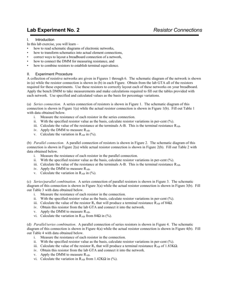
Lab Experiment No. 2
Resistor Connections
I.
Introduction
In this lab exercise, you will learn –
• how to read schematic diagrams of electronic networks,
• how to transform schematics into actual element connections,
• correct ways to layout a breadboard connection of a network,
• how to connect the DMM for measuring resistance, and
• how to combine resistors to establish terminal equivalence.
II. Experiment Procedure
A collection of resistive networks are given in Figures 1 through 6. The schematic diagram of the network is shown
in (a) while the resistor connection is shown in (b) in each Figure. Obtain from the lab GTA all of the resistors
required for these experiments. Use these resistors to correctly layout each of these networks on your breadboard.
Apply the bench DMM to take measurements and make calculations required to fill out the tables provided with
each network. Use specified and calculated values as the basis for percentage variations.
(a) Series connection. A series connection of resistors is shown in Figure 1. The schematic diagram of this
connection is shown in Figure 1(a) while the actual resistor connection is shown in Figure 1(b). Fill out Table 1
with data obtained below.
i. Measure the resistance of each resistor in the series connection.
ii. With the specified resistor value as the basis, calculate resistor variations in per-cent (%).
iii. Calculate the value of the resistance at the terminals A-B. This is the terminal resistance RAB.
iv. Apply the DMM to measure RAB.
v. Calculate the variation in RAB in (%).
(b) Parallel connection. A parallel connection of resistors is shown in Figure 2. The schematic diagram of this
connection is shown in Figure 2(a) while actual resistor connection is shown in Figure 2(b). Fill out Table 2 with
data obtained below.
i. Measure the resistance of each resistor in the parallel connection.
ii. With the specified resistor value as the basis, calculate resistor variations in per-cent (%).
iii. Calculate the value of the resistance at the terminals A-B. This is the terminal resistance RAB.
iv. Apply the DMM to measure RAB.
v. Calculate the variation in RAB in (%).
(c) Series/parallel combination. A series connection of parallel resistors is shown in Figure 3. The schematic
diagram of this connection is shown in Figure 3(a) while the actual resistor connection is shown in Figure 3(b). Fill
out Table 3 with data obtained below.
i. Measure the resistance of each resistor in the connection.
ii. With the specified resistor value as the basis, calculate resistor variations in per-cent (%).
iii. Calculate the value of the resistor Rx that will produce a terminal resistance RAB of 84Ω.
iv. Obtain this resistor from the lab GTA and connect it into the network.
v. Apply the DMM to measure RAB.
vi. Calculate the variation in RAB from 84Ω in (%).
(d) Parallel/series combination. A parallel connection of series resistors is shown in Figure 4. The schematic
diagram of this connection is shown in Figure 4(a) while the actual resistor connection is shown in Figure 4(b). Fill
out Table 4 with data obtained below.
i. Measure the resistance of each resistor in the connection.
ii. With the specified resistor value as the basis, calculate resistor variations in per-cent (%).
iii. Calculate the value of the resistor Rx that will produce a terminal resistance RAB of 1.83KΩ.
iv. Obtain this resistor from the lab GTA and connect it into the network.
v. Apply the DMM to measure RAB.
vi. Calculate the variation in RAB from 1.42KΩ in (%).
(e) Combination 1 (Combo 1) connection. A combination connection of resistors in series and parallel is shown in
Figure 5. The schematic diagram of this connection is shown in Figure 5(a) while the actual resistor connection is
shown in Figures 5(b). Fill out Table 5 with data obtained below.
i. Measure the resistance of each resistor in the connection.
ii. With the specified resistor value as the basis, calculate the resistor variation in per-cent (%).
iii. Calculate the value of the resistance at the terminals A-B. This is the terminal resistance RAB.
iv. Apply the DMM to measure RAB.
v. Calculate the variation in RAB in (%).
(f) Combination 2 (Combo 2) connection. Yet another combination connection of resistors in series and parallel is
shown in Figure 6. The schematic diagram of this connection is shown in Figure 6(a) while the actual resistor
connection is shown in Figures 6(b). Fill out Table 6 with data obtained below.
i. Measure the resistance of each resistor in the connection.
ii. With the specified resistor value as the basis, calculate the resistor variation in per-cent (%).
iii. Calculate the value of the resistance at the terminals A-B. This is the terminal resistance RAB.
iv. Apply the DMM to measure RAB.
v. Calculate the variation in RAB in (%).
III. Lab Report
The report for this lab experiment must be word-processed and contain the following items –
• Title Page.
• Introduction.
• Procedure.
• Results.
• Discussions.
(a) Suggest useful applications for the connections studied in this experiment.
• Conclusion. Provide detailed comments and discussions on the items listed below for each resistor network.
(a) Are all resistors within tolerance? List those that are not.
(b) Account for the difference between measured R AB and calculated RAB (that is, the calculated variation or
tolerance of RAB).
(c) Explain how the variation in RAB corresponds to resistor tolerance.
(d) Explain how close the calculated values of Rx in the series/parallel and parallel/series connections are to
standard resistor values. Consider resistor tolerance.
• Appendix.
• References.
Series Connection
1
R1
1
R2
2
A
3.9K
A
R1
2
R2
2K
R3
RAB
8.2K
5.1K
RAB
R3
1.2K
B
4
R5
R4
3
B
R5
R4
4
(a)
(b)
Figure 1
(a) Schematic for the series connection
(b) Component connection diagram
Table 1
Series connection
Resistor
(Ri)
Specified value
(Ω)
R1
3.9K
R2
2K
R3
5.1K
R4
1.2K
R5
8.2K
Terminal
resistance
Calculated value
(Ω)
RAB
Measured value
(Ω)
Variation
(%)
Measured value
(Ω)
Variation
(%)
3
Parallel Connection
A
A
R1
R2
R4
R3
R5
RAB
RAB
10K
7.5K
15K
3.3K
R1
R2
R3
2.2K
B
B
(a)
(b)
Figure 2
(a) Schematic for the parallel connection
(b) Component connection diagram
Table 2
Parallel connection
Resistor
(Ri)
Specified value
(Ω)
R1
10K
R2
7.5K
R3
15K
R4
3.3K
R5
2.2K
Terminal
resistance
Calculated value
(Ω)
RAB
Measured value
(Ω)
Variation
(%)
Measured value
(Ω)
Variation
(%)
R4
R5
Series/Parallel Connection
R6
R1
15
Rx
A
2
R3
75
30
62
R4
R6
R3
R1
R7
3
1
A
12
27
82
R2
56
R8
RAB
Rx
R7
2
1
R2
R9
B
(b)
(a)
Figure 3
(a) Schematic for the series/parallel connection
(b) Component connection diagram
Table 3
Series/parallel connection
Resistor
(Ri)
Specified value
(Ω)
R1
15
R2
12
R3
30
R4
27
R5
56
R6
75
R7
62
R8
82
R9
91
Measured value
(Ω)
Variation
(%)
Measured value
(Ω)
Variation
(%)
Rx
Terminal
resistance
Specified value
(Ω)
RAB
84
R8
R9
91
B
3
R5
RAB
R5
R4
Parallel/Series Connection
R6
R6
7.5K
4
R3
A
R3
RAB
B
3.0K
4
R1
A
R1
Rx
R2
1.5K
2
1
2.7K
5
3
8.2K
R4
1.2K
R7
2
R8
RAB
1
Rx
5.6K
5
R4
R2
R5
R7
6.2K
3
R8
6
B
R9
9.1K
6
R5
R9
(a)
(b)
Figure 4
(a) Schematic for the parallel/series connection
(b) Component connection diagram
Table 4
Parallel/series connection
Resistor
(Ri)
Specified value
(Ω)
R1
1.5K
R2
1.2K
R3
3K
R4
2.7K
R5
5.6K
R6
7.5K
R7
6.2K
R8
8.2K
R9
9.1K
Measured value
(Ω)
Variation
(%)
Measured value
(Ω)
Variation
(%)
Rx
Terminal
resistance
Specified value
(Ω)
RAB
1.83K
Combo 1 Connection
R1
R9
1
5
A
1.2K
200
R3
R4
R5
1.2K
3.6K
R11
2
R15
6
R12
1.3K
R6
RAB
1K
1.8K
R13
1.5K
7
R8
2.2K
1.3K
R14
1K
2.2K
300
B
R2
4
R10
Figure 5
(a) Schematic for Combo 1 connection
(b) Component connection diagram
8
9
3K
3
R7
2K
R16
1K
Table 5
Combo 1 connection
Resistor
(Ri)
Specified value
(Ω)
R1
200
R2
1.3K
R3
3.6K
R4
1.2K
R5
1.8K
R6
1.3K
R7
2.2K
R8
2.2K
R9
1.2K
R10
300
R11
1K
R12
1.5K
R13
3K
R14
1K
R15
2K
R16
1K
Terminal
resistance
Calculated value
(Ω)
RAB
Measured value
(Ω)
Variation
(%)
Measured value
(Ω)
Variation
(%)
Combo 2 connection
R1
1
A
47K
R2
R3
120K
R9
10K
30K
R13
R14
100K
2
4
RAB
R4
R5
R10
30K
20K
7
R11
100K
R15
300K
3
8
5
R6
R7
15K
15K
30K
R12
15K
R8
B
22K
6
Figure 6
(a) Schematic for Combo 2 connection
(b) Component connection diagram
R16
75K
150K
Table 6
Combo 2 connection
Resistor
(Ri)
Specified value
(Ω)
R1
47K
R2
30K
R3
120K
R4
20K
R5
30K
R6
15K
R7
30K
R8
22K
R9
10K
R10
300K
R11
100K
R12
15K
R13
100K
R14
150K
R15
15K
R16
75K
Terminal
resistance
Calculated value
(Ω)
RAB
Measured value
(Ω)
Variation
(%)
Measured value
(Ω)
Variation
(%)