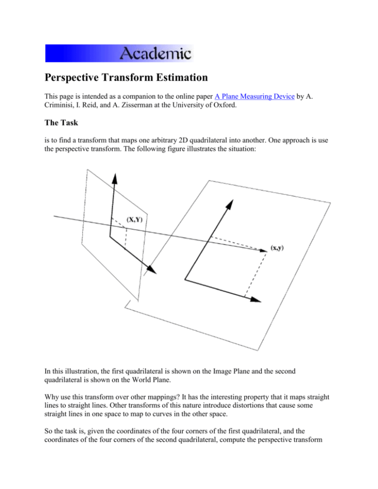
Perspective Transform Estimation
This page is intended as a companion to the online paper A Plane Measuring Device by A.
Criminisi, I. Reid, and A. Zisserman at the University of Oxford.
The Task
is to find a transform that maps one arbitrary 2D quadrilateral into another. One approach is use
the perspective transform. The following figure illustrates the situation:
In this illustration, the first quadrilateral is shown on the Image Plane and the second
quadrilateral is shown on the World Plane.
Why use this transform over other mappings? It has the interesting property that it maps straight
lines to straight lines. Other transforms of this nature introduce distortions that cause some
straight lines in one space to map to curves in the other space.
So the task is, given the coordinates of the four corners of the first quadrilateral, and the
coordinates of the four corners of the second quadrilateral, compute the perspective transform
that maps a new point in the first quadrilateral onto the appropriate position on the second
quadrilateral.
Deriving the Homographic Transform
The solution is stated in Section 3.1 of the paper, but the derivation is a bit lacking. I will briefly
sketch the derivation here to make the solution more appetizing. We start with the claim that the
camera model could be written as X=Hx, where X is vector of world plane coordinates, x is the
vector of image plane coordinates, and H is a matrix transform. We can write the this form out in
more detail as:
Then if we realize that W is actually:
we can rewrite the equation in a way that exposes its true non-linear form where the numerator
supplies the parameters needed for affine transformation, and the denominator allows for the
non-linear effect of perspective:
This is equivalent to the possibly more familiar, non-vector form of the perspective transform:
By multiplying each side of the equation by the denominator we get:
and multiplying through by X and Y gives us:
Now we isolate the naked X and Y terms on the left:
If we add in some zero terms:
then it becomes more clear that this is the product of a matrix and a vector:
and we have reached the previously mysterious point that Criminisi leaps to in a single step:
The Solution
The form of this equation is Ax=b, and it can be solved by several methods that amount to a least
squares estimation of the parameter vector x that satisfies the linear relationship between the
matrix A and the vector of output coordinates B. The simplest, although not the most
numerically stable, is to use the pseudo-inverse:
The rest of the Criminisi paper discusses issues of measurement noise and estimation uncertainty
that are important when choosing the right estimation method for a given application.
The Code
This code implements this solution in Matlab for the case of mapping an user selected
quadrilateral onto a rectangle.
hold off
axis([0 640 0 480 ])
[X,Y] = ginput(4)
plot([X;X(1)],[Y;Y(1)],'r')
hold
plot([0 0 640 640 0], [0 480 480 0 0],'b')
axis([ -100 900 -100 580 ])
Xp=[0;
0; 640; 640];
Yp=[0; 480; 480;
0];
B = [ X Y ones(size(X)) zeros(4,3)
-X.*Xp -Y.*Xp ...
zeros(4,3)
X Y ones(size(X)) -X.*Yp -Y.*Yp ];
B = reshape (B', 8 , 8 )';
D = [ Xp , Yp ];
D = reshape (D', 8 , 1 );
l = inv(B' * B) * B' * D;
A = reshape([l(1:6)' 0 0 1 ],3,3)';
C = [l(7:8)' 1];
while 1 ,
[x1,y1]=ginput(1);
[x2,y2]=ginput(1);
for u=0:.1:1,
x = u*x1+(1-u)*x2;
y = u*y1+(1-u)*y2;
plot(x,y,'xr'); t=A*[x;y;1]/(C*[x;y;1]);plot(t(1),t(2),'ob')
end
end
Screen Shots
Acknowledgments
Many thanks to Stephen Intille , Lee Campbell, Dave Berger, Sumit Basu, and Tony Jebara for
their advise on this topic.
Go Up a Level
"Christopher R. Wren" <wren@media.mit.edu>
$Id: interpolator.html,v 1.2 1998/12/10 16:15:28 cwren Exp cwren $
�1998 Christopher R. Wren.
Use of this material without prior written consent is strictly forbidden.