A Brief Introduction to Bayesian Statistics
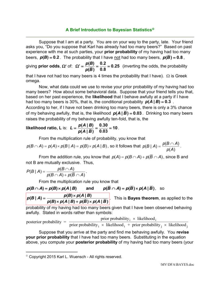
Suppose that I am at a party. You are on your way to the party, late. Your friend
asks you, “Do you suppose that Karl has already had too many beers?” Based on past
experience with me at such parties, your prior probability of my having had too many
beers, p(B) 0.2 . The probability that I have not had too many beers, p(B ) 0.8 ,
p(B) 0.2
0.25 (inverting the odds, the probability
giving prior odds, of:
p(B ) 0.8
that I have not had too many beers is 4 times the probability that I have). is Greek
omega.
Now, what data could we use to revise your prior probability of my having had too
many beers? How about some behavioral data. Suppose that your friend tells you that,
based on her past experience, the likelihood that I behave awfully at a party if I have
had too many beers is 30%, that is, the conditional probability p( A | B) 0.3 .
According to her, if I have not been drinking too many beers, there is only a 3% chance
of my behaving awfully, that is, the likelihood p( A | B ) 0.03 . Drinking too many beers
raises the probability of my behaving awfully ten-fold, that is, the
p( A | B) 0.30
10 .
likelihood ratio, L is: L
p( A | B ) 0.03
From the multiplication rule of probability, you know that
p(B A) p( A) p(B | A) p(B ) p( A | B ) , so it follows that p(B | A)
p(B A)
.
p( A)
From the addition rule, you know that p( A) p(B A) p(B A) , since B and
not B are mutually exclusive. Thus,
p(B A)
.
P (B | A )
p(B A) p(B A)
From the multiplication rule you know that
p(B A) p(B) p( A | B)
and
p(B A) p(B ) p( A | B ) , so
p(B) p( A | B)
. This is Bayes theorem, as applied to the
p(B) p( A | B) p(B ) p( A | B )
probability of my having had too many beers given that I have been observed behaving
awfully. Stated in words rather than symbols:
prior probability i likelihood i
posterior probability =
prior probability i likelihood i + prior probability j likelihood j
p(B | A)
Suppose that you arrive at the party and find me behaving awfully. You revise
your prior probability that I have had too many beers. Substituting in the equation
above, you compute your posterior probability of my having had too many beers (your
Copyright 2015 Karl L. Wuensch - All rights reserved.
\MV\DFA\BAYES.doc
2
revised opinion, after considering the new data, my having been found to be behaving
awfully):
.2(.3)
p(B | A)
0.714 . Of course, that means that your posterior probability
.2(.3) .8(.03)
that I have not had too many beers is 1 - 0.714 = 0.286. The posterior odds
0.714
2.5 . You now think the probability that I have had too many beers is 2.5
0.286
times the probability that I have not had too many beers.
Note that Bayes theorem can be stated in terms of the odds and likelihood ratios:
the posterior odds equals the product of the prior odds and the likelihood ratio.
Ω Ω L : 2.5 = 0.25 x 10.
Bayesian Hypothesis Testing
You have two complimentary hypotheses, H0, the hypothesis that I have not had
too many beers, and H1, the hypothesis that I have had too many beers. Letting D
stand for the observed data, Bayes theorem then becomes:
P (H 0 D )
P (H 0 ) P ( D | H 0 )
P (H 0 | D )
, and
P (D )
P (H0 ) P (D | H0 ) P (H1 ) P (D | H1 )
P (H1 | D )
P (H1 D )
P (H1 ) P (D | H1 )
.
P (D )
P (H0 ) P (D | H0 ) P (H1 ) P (D | H1 )
The P(H0|D) and P(H1|D) are posterior probabilities, the probability that the null is
true given tP p(H1) are prior probabilities, the probability that the null or the alternative is
true prior to considering the new data. The P(D|H0) and P(D|H1) are the likelihoods, the
probabilities of the data given one or the other hypothesis.
P (H1 | D ) P (H1 ) P (D | H1 )
As before, L , that is,
P (H 0 | D ) P (H 0 ) P (D | H 0 )
In classical hypothesis testing, one considers only P(D|H0), or more precisely, the
probability of obtaining sample data as or more discrepant with null than are those on
hand, that is, the obtained significance level, p, and if that p is small enough, one rejects
the null hypothesis and asserts the alternative hypothesis. One may mistakenly believe
e has estimated the probability that the null hypothesis is true, given the obtained data,
but e has not done so. The Bayesian does estimate the probability that the null
hypothesis is true given the obtained data, P(H0|D), and if that probability is sufficiently
small, e rejects the null hypothesis in favor of the alternative hypothesis. Of course,
how small is sufficiently small depends on an informed consideration of the relative
seriousness of making one sort of error (rejecting H0 in favor of H1) versus another sort
of error (retaining H0 in favor of H1).
Suppose that we are interested in testing the following two hypotheses about the
IQ of a particular population H: μ = 100 versus H1: μ = 110. I consider the two
hypotheses equally likely, and dismiss all other possible values of μ, so the prior
probability of the null is .5 and the prior probability of the alternative is also .5.
3
I obtain a sample of 25 scores from the population of interest. I assume it is
normally distributed with a standard deviation of 15, so the standard error of the mean is
15/5 = 3. The obtained sample mean is 107. I compute for each hypothesis
M i
zi
. For H the z is 2.33. For H1 it is -1.00. The likelihood p(D|H0) is obtained
M
by finding the height of the standard normal curve at z = 2.33 and dividing by 2 (since
2
ez / 2
there are two hypotheses). The height of the normal curve can be found by
,
2
where pi is approx. 3.1416, or you can use a normal curve table, SAS, SPSS, or other
statistical program. Using PDF.NORMAL(2.333333333333,0,1) in SPSS, I obtain
.0262/2 = .0131. In the same way I obtain the likelihood p(D|H1) = .1210. The
P(D) P(H0 ) P(D | H0 ) P(H1) P(D | H1) .5(.0131) .5(.121) .06705 . Our revised,
posterior probabilities are:
.5(.1210)
P (H0 ) P (D | H0 ) .5(.0131)
.9023 .
P (H 0 | D )
.0977 , and P (H1 | D )
.06705
P (D )
.06705
Before we gathered our data we thought the two hypotheses equally likely, that
is, the odds were 1/1. Our posterior odds are .9023/.0977 = 9.24. That is, after
gathering our data we now think that H1 is more than 9 times more likely than is H.
P (D | H1 ) .1210
9.24 . Multiplying the prior odds ratio (1)
The likelihood ratio
P (D | H0 ) .0131
by the likelihood ratio gives us the posterior odds. When the prior odds = 1 (the null and
the alternative hypotheses are equally likely), then the posterior odds is equal to the
likelihood ratio. When intuitively revising opinion, humans often make the mistake of
assuming that the prior probabilities are equal.
If we are really paranoid about rejecting null hypotheses, we may still retain the
null here, even though we now think the alternative about nine times more likely.
Suppose we gather another sample of 25 scores, and this time the mean is 106. We
can use these new data to revise the posterior probabilities from the previous analysis.
For these new data, H the z is 2.00 for H, and -1.33 for H1. The likelihood P(D|H0) is
.0540/2 = .0270 and the likelihood P(D|H1) is .1640/2 = .0820. The
P(D) P(H0 ) P(D | H0 ) P(H1) P(D | H1) .0977(.0270) .9023(.0820) .07663 . The
newly revised posterior probabilities are
P (H0 ) P (D | H0 ) .0977(.0270)
P (H 0 | D )
.0344 , and
P (D )
.07663
.9023(.0820)
P (H1 | D )
.9655 .
.07663
The likelihood ratio is .082/.027 = 3.037. The newly revised posterior odds is
.9655/.0344= 28.1. The prior odds 9.24, times the likelihood ratio, 3.037, also gives the
posterior odds, 9.24(3.037) = 28.1. With the posterior probability of the null at .0344, we
should now be confident in rejecting it.
The Bayesian approach seems to give us just want we want, the probability of
the null hypothesis given our data. So what’s the rub? The rub is, to get that posterior
4
probability we have to come up with the prior probability of the null being true. If you
and I disagree on that prior probability, given the same data, we arrive at different
posterior probabilities. Bayesians are less worried about this than are traditionalists,
since the Bayesian thinks of probability as being subjective, one’s degree of belief about
some hypothesis, event, or uncertain quantity. The traditionalist thinks of a probability
as being an objective quantity, the limit of the relative frequency of the event across an
uncountably large number of trials (which, of course, we can never know, but we can
estimate by rational or empirical means). Advocates of Bayesian statistics are often
quick to point out that as evidence accumulates there is a convergence of the posterior
probabilities of those started with quite different prior probabilities.
Bayesian Confidence Intervals
In Bayesian statistics a parameter, such as μ, is thought of as a random variable
with its own distribution rather than as a constant. That distribution is thought of as
representing our knowledge about what the true value of the parameter may be, and the
mean of that distribution is our best guess for the true value of the parameter. The
wider the distribution, the greater our ignorance about the parameter. The precision
(prc) of the distribution is the inverse of its variance, so the greater the precision, the
greater our knowledge about the parameter.
Our prior distribution of the parameter may be noninformative or informative. A
noninformative prior will specify that all possible values of the parameter are equally
likely. The range of possible values may be fixed (for example, from 0 to 1 for a
proportion) or may be infinite. Such a prior distribution will be rectangular, and if the
range is not fixed, of infinite variance. An informative prior distribution specifies a
particular nonuniform shape for the distribution of the parameter, for example, a
binomial, normal, or t distribution centered at some value. When new data are
gathered, they are used to revise the prior distribution. The mean of the revised
(posterior) distribution becomes our new best guess of the exact value of the parameter.
We can construct a Bayesian confidence interval and opine that the probability that the
true value of the parameter falls within that interval is cc, where cc is the confidence
coefficient (typically 95%).
Suppose that we are interested in the mean of a population for which we confess
absolute ignorance about the value of μ prior to gathering the data, but we are willing to
assume a normal distribution. We obtain 100 scores and compute the sample mean to
be 107 and the sample variance 200. The precision of this sample result is the inverse
of its squared standard error of the mean. The standard error of the mean is
200 / 100 2 = SEM2 = 2. Precision = ½ = .5.
SEM s 2 / N , so SEM2 = s2/N, and the inverse of SEM2 is N/s2 = precision.
The 95% Bayesian confidence interval is identical to the traditional confidence
interval, that is, M 1.96sM 107 1.96 2 107 2.77 104.23 109.77 .
Now suppose that additional data become available. We have 81 scores with a
mean of 106, a variance of 243, and a precision of 81/243 = 1/3. Our prior distribution
has (from the first sample) a mean of 107 and a precision of .5. Our posterior
distribution will have a mean that is a weighted combination of the mean of the prior
5
distribution and that of the new sample. The weights will be based on the precisions:
prc1
prcS
.5
.3
2
1
MS
107
106 106.6 .
prc1 prcS
prc1 prcS
.5 . 3
.5 . 3
The precision of the revised (posterior) distribution for μ is simply the sum of the
prior and sample precisions: prc 2 prc1 prcS .5 . 3 .8 3 . The variance of the
revised distribution is just the inverse of its precision, 1.2. Our new Bayesian
confidence interval is 2 1.96 2 106.6 1.96 1.2 106.6 2.15 104.46 108.75 .
Of course, if more data come in, we revise our distribution for μ again. Each time
the width of the confidence interval will decline, reflecting greater precision, more
knowledge about μ.
Visualization of Bayes Theorem
Copyright 2015 Karl L. Wuensch - All rights reserved.
