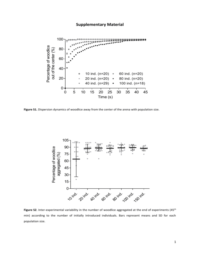
Supplementary Material
Percentage of woodlice
out of the center (%)
100
80
60
40
10 ind. (n=20)
20 ind. (n=20)
40 ind. (n=29)
20
60 ind. (n=20)
80 ind. (n=20)
100 ind. (n=18)
0
0
5
10
15
20 25 30
Time (s)
35
40
45
Figure S1. Dispersion dynamics of woodlice away from the center of the arena with population size.
Percentage of woodlice
aggregated (%)
105
90
75
60
45
30
15
d.
in
d.
15
0
in
10
0
in
d.
80
in
d.
60
in
d.
40
in
d.
20
10
in
d.
0
Figure S2. Inter-experimental variability in the number of woodlice aggregated at the end of experiments (45th
min) according to the number of initially introduced individuals. Bars represent means and SD for each
population size.
1
Average number of
secondary aggregates
per experiment
Average number of
woodlice per
secondary aggregate
Average lifetime of
secondary aggregates
(min)
10
woodlice
(n=20)
20
woodlice
(n=20)
40
woodlice
(n=28)
60
woodlice
(n=20)
80
woodlice
(n=20)
100
woodlice
(n=18)
150
woodlice
(n=15)
0.05
0.25
0.92
0.9
0.55
0.88
-
2
2.3 ± 0.2
4.2 ± 2.0
4.9 ± 3.0
5.0 ± 2.0
4.0 ± 1.5
-
6
13.4 ± 6.2
14.6 ± 12.8
8.1 ± 7.3
7.3 ± 5.0
6.4 ± 3.8
-
Table S1. Analysis of secondary aggregates outside of the shelters. There is no difference between the number
of secondary aggregates produced by population size, except for the 10 woodlice group significantly lower than
the 40, 60 and 100 woodlice groups, and the 20 woodlice group significantly lower than the 60 and 100
woodlice groups (Kruskal-Wallis and Dunn test; p<0.001; KW=26.016). There is no difference between the
average number of woodlice per aggregate (means ± SD), except at 20 woodlice, which differs from 60 and 80
woodlice (Kruskal-Wallis and Dunn test; p=0.0101; KW=15.070). There is a difference between the average
lifetimes of the secondary aggregates (means ± SD), but the Kruskal-Wallis and Dunn post-test does not detect
any pairwise differences between the groups (p=0.0165; KW=13.861).
1.0
Fraction of experiments
***
0.8
0.6
0.4
0.2
0.0
<
ost
M
s
Les
>
ost
s
Les
M
Figure S3. Fraction of experiments (n=56) where the final aggregate in the most-filled shelter presents a smaller
length/width ratio than that in the least-filled shelter just before irreversible selection of the shelters, and vice
versa. The difference between the fractions is significant (Chi-square test, p<0.0001). On average, the value of
the length/width ratio of the aggregate in the most-filled shelter is 2.4 (+/- 0.96), which is significantly lower
(Wilcoxon match-paired test, p= 0.0007) than that in the least-filled shelter (2.9 +/- 1.12).
2
Figure S4: Conformation of aggregates under shelters
In this section, we consider the spatiotemporal conformation of the individuals aggregated under the
shelters.
First, the surface area of the aggregate (S) increases with the number of individuals inside (N) in
accordance with the non-linear relationships of S= 0.6N0.77 (R²=0.8284) and S= 0.9N0.65 (R²=0.9413) for
the most- and least-filled shelters, respectively (Fig. S4A). A one-way ANCOVA test of the logarithmic
data indicates an equality between the two slopes (F=0.4706, p=0.4913) and a difference between
the adjusted means of the regressions (F= 8.088, p= 0.0051). The mean fitting of the coupled data for
Ln (Surface area)
the most- and least-filled shelters gives the relationship: S= 0.6N0.75 (R²=0.8955).
4.0
3.5
3.0
2.5
2.0
1.5
1.0
0.5
0.0
-0.5
-1.0
-1.5
Most-filled shelter
Least-filled shelter
1
2
3
4
Ln (number of individuals)
5
Figure S4A. Logarithmic relationship between the total surface area of the aggregates (cm²) and the number of
individuals inside the most- or least-filled shelter at the end of the binary choice tests (45th min). All of the
experimental conditions are pooled.
Secondly, the measurement of surface area occupied by the aggregate under the shelter reaching
the most of individuals (only under the shelter, regardless of the overflow) shows the gradual
increase of the shelter filling according to the density, up to more than 90% when 100 or 150
woodlice are introduced (Fig. 5B, 6A, S4B). At this stage, we can talk of a saturation of the shelter.
This saturation is counterbalanced by the increasing overflowing of the aggregate beyond limits of
the shelter, reaching almost half (46%) of the total size of the aggregate with 100 and 150 woodlice
(Fig. 5B, 6B, S4C).
Aggregates under the most or the least filled shelter of the binary choice test present similar spatial
conformation at the end of experiments. Indeed, regardless of the number of individuals, the
aggregates under the both shelters present similar surface area pattern (Fig. S4A) and similar shape
(i.e., with similar shelter filling (Fig. 6A, S4B) and similar shelter overflowing (Fig. 6B, S4C)).
3
Most-filled shelter
C
100
Shelter overflowing (%)
80
60
40
20
Most-filled shelter
80
60
40
20
in
d.
d.
0
15
0
10
20 ind
in .
d.
40
in
d.
60
in
d.
80
in
d.
10
0
in
d.
0
Least-filled shelter
in
Shelter filling (%)
100
15
0
Least-filled shelter
10
20 ind
in .
d.
40
in
d.
60
in
d.
80
in
d.
10
0
in
d.
B
Figure S4B. Percentage of the most- and least-filled shelters that are filled by the aggregate (expressed as the
percentage of the surface area occupied by the aggregate under the shelter at the end of the experiments)
according to the number of initially introduced woodlice. The error bars represent the standard deviations.
Figure S4C. Surface area of the aggregate overflowing from the most- and least-filled shelters (expressed as the
percent of the total surface area of the aggregate at the end of the experiments) according to the number of
initially introduced woodlice. The error bars represent the standard deviations.
In addition, the surface area per individual decreases with the number of individuals in the aggregate
(Fig. S4D), as demonstrated previously (Broly et al., 2014). Here, we show that the surface area per
individual also decreases independently of the number of woodlice with the duration of the
experiment (Fig. S4D, E). In other words, group compaction increases with both the number of
conspecifics and time. The gain in compactness is of 35% between the 5 first minutes and the end of
experiments (Fig. S4E). Finally, the length/width ratio of the aggregate decreases during the
experiment (Fig. S4F). In other words, the aggregate first grows in length (due to the strong behavior
of the woodlice to follow the edge of the arena) and then progressively grows in width, which
indicates a reduction of the effect of the edge on the group and a spatiotemporal reorganization of
the woodlice toward the center of the arena. This spatiotemporal compaction of the woodlice leads
to a reduced surface area/volume ratio of the aggregate and therefore leads to reduce the individual
exchanges with the environment as body water loss (see Broly et al. 2014).
4
E
D
Surface area (cm²) / Ind.
Surface area (cm²) / Ind.
0.6
0.4
0.2
0.0
0
0.45
0.40
0.35
0.30
0.25
0.20
0.15
0.10
0.05
0.00
20
40
60
80
100
Number of individuals in the aggregate
0
5
10
15
20 25 30
Time (min)
35
40
45
Figure S4D. Relationship between the surface area (in cm²) per individual and the number of individuals in the
aggregate, at the end of the experiments (in grey, which includes data at the 45th min from experiments with
10 to 150 ind.) or during the experiments (in black, which includes data from experiments with 100 ind. at
different times). The grey scatter plot is fitted by S= 0.896N -0.3118 (R²= 0.4339), and the black scatter plot by S=
0.5099N-0.1916 (R²= 0.4026). There is a significant difference between the slopes of the two curves (one-way
ANCOVA, F= 8.647, p= 0.00356).
Figure S4E. Relationship between the surface area (in cm²) per individual in the aggregate and the duration of
experiment (in experiments with 100 woodlice). The surface area per individual (S) decreases with time (t),
following S= 0.4121t-0.1877 (R²= 0.958). The error bars represent the standard deviations.
G
Lenght/Width ratio
5
4
3
2
1
0
0
5
10 15 20 25 30 35 40 45 50
Time (min)
Figure S4F. Schematic representation of the aggregate centered under shelter and the location of
measurements.
Figure S4G. Relationship between the shape of the aggregate (length/width ratio) and the duration of the
experiment (in experiments with 100 woodlice).
The ratio (R) decreases with time (t), according to R= 4.226t-0.1687 (R²= 0.9431). The gain in compactness is of
29% between the 5 first minutes and the end of experiments. The error bars represent the standard deviations.
5
500
10
a
10
b
y= 0.1071x
400
8
400
8
300
6
300
6
200
4
200
4
100
2
100
2
0
4000
0
0
0
50
1000
2000
3000
10
c
8
40
y= 0.7213x
6
4
y= 0.1225x
2
0
150
0
160
25
50
75
100
125
10
e
140
2000
0
4000
3000
10
d
60
8
6
40
y= 0.6203x
30
4
20
10
0
70
1000
50
30
20
0
2
10
y= 0.1564x
0
0
160
8
100
6
80
50
75
100
125
150
0
175
10
f
140
120
25
8
120
100
6
80
y= 0.4112x
60
40
4
2
20
0
0
80
150
300
450
8
60
6
40
4
y= 0.1153x
y= 0.5756x
2
0
0
0
50
100
150
200
2
250
300
y= 0.1360x
0
0
10
20
40
600
g
4
y= 0.3822x
20
y= 0.1204x
0
60
Number of individuals under shleter
Cumulative number of entries into shelter
500
y= 0.1152x
225
200
175
150
125
100
75
50
25
0
150
0
450
300
h
y= 0.5042x
10
8
y= 0.1173x
6
4
2
0
0
300
600
900
1200
1500
Cumulative number of individuals outside shelter
Figure S5. Cumulative number of entries into a shelter according to the cumulative number of individuals
outside shelter in two experiments without aggregation (a, b), five experiments presenting fast and stable
aggregation (c, d, e, f, g), and an experiment with aggregation obtained after 30 min (h). The number of
individuals aggregated in the shelter is shown by the right axis (grey points). The curve may be fit by one or two
linear regression(s); the red line fits phases where mechanisms of amplification of the aggregation process are
not at work, while in contrast, the blue line fits the phase where attraction occurs (increasing slopes).
6
120
a
100
80
60
0
1
2
3 4 5 6 7 8
Number of individuals
9 10 11
Figure S6. Values of parameter a in equation (6) that fit the residence time for each group size. The values of a
according to the number of individuals under shelter (N) are fitted by a linear regression: a= -0.5382(±0.4345)N
+ 103.6(±2.696) (r²= 0.1610). An F test on the linear regression indicates the slope for a does not deviate from
zero (F=1.535, p=0.2505).
7