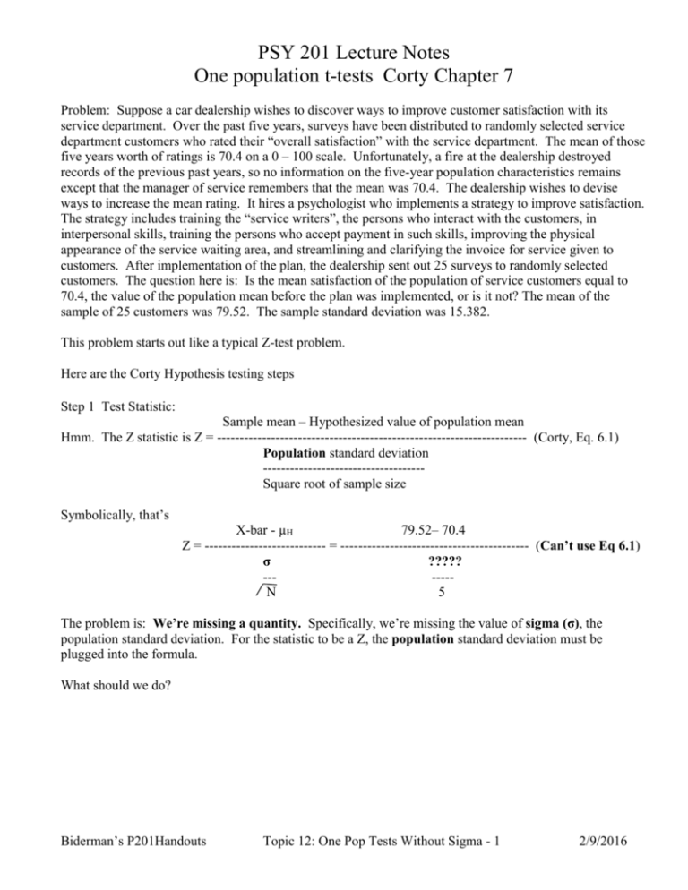
PSY 201 Lecture Notes
One population t-tests Corty Chapter 7
Problem: Suppose a car dealership wishes to discover ways to improve customer satisfaction with its
service department. Over the past five years, surveys have been distributed to randomly selected service
department customers who rated their “overall satisfaction” with the service department. The mean of those
five years worth of ratings is 70.4 on a 0 – 100 scale. Unfortunately, a fire at the dealership destroyed
records of the previous past years, so no information on the five-year population characteristics remains
except that the manager of service remembers that the mean was 70.4. The dealership wishes to devise
ways to increase the mean rating. It hires a psychologist who implements a strategy to improve satisfaction.
The strategy includes training the “service writers”, the persons who interact with the customers, in
interpersonal skills, training the persons who accept payment in such skills, improving the physical
appearance of the service waiting area, and streamlining and clarifying the invoice for service given to
customers. After implementation of the plan, the dealership sent out 25 surveys to randomly selected
customers. The question here is: Is the mean satisfaction of the population of service customers equal to
70.4, the value of the population mean before the plan was implemented, or is it not? The mean of the
sample of 25 customers was 79.52. The sample standard deviation was 15.382.
This problem starts out like a typical Z-test problem.
Here are the Corty Hypothesis testing steps
Step 1 Test Statistic:
Sample mean – Hypothesized value of population mean
Hmm. The Z statistic is Z = --------------------------------------------------------------------- (Corty, Eq. 6.1)
Population standard deviation
-----------------------------------Square root of sample size
Symbolically, that’s
X-bar - µH
79.52– 70.4
Z = --------------------------- = ------------------------------------------ (Can’t use Eq 6.1)
σ
?????
------N
5
The problem is: We’re missing a quantity. Specifically, we’re missing the value of sigma (σ), the
population standard deviation. For the statistic to be a Z, the population standard deviation must be
plugged into the formula.
What should we do?
Biderman’s P201Handouts
Topic 12: One Pop Tests Without Sigma - 1
2/9/2016
The test statistic problem
This problem was faced by statisticians of old (who would now be very old statisticians.)
They wanted to compute a Z statistic but did not know the value of the population standard deviation.
In fact, this is the situation we’ll most likely face.
If we’re so ignorant of the characteristics of a population that we don’t know its mean, how in earth could
we know its standard deviation?
The answer is: We couldn’t. We need to find a way of testing such hypotheses without having to know the
value of the population standard deviation.
Why do we even care?
We care because we can’t determine the p-value necessary for making a decision. The determination of
the p-value depends on the use of the Normal Distribution tables. But if we don’t have a Z statistic, we
can’t use the Normal Distribution tables.
Two possible solutions
Solution 1: Take a large sample and use the sample standard deviation as a substitute for the population
standard deviation.
This is what statisticians of old did in the early 1900s. They took samples of 200+, used the sample
standard deviation in place of the population standard deviation in the formula, and pretended that they had
a Z statistic. They then used the Normal distribution tables to determine p-values.
This procedure was technically incorrect, since the number they put in the Z-statistic formula was NOT the
actual population standard deviation but a sample quantity.
But since the sample sizes they used were very large, the value they substituted was probably quite close to
the true value, and they probably computed p-values that were very close to the correct ones.
So why not just keep on doing this – taking huge samples and pretending the statistic is a Z.
a. Huge samples cost a lot in terms of $ and time.
b. It just isn’t right.
Biderman’s P201Handouts
Topic 12: One Pop Tests Without Sigma - 2
2/9/2016
Solution 2. Figure out the correct sampling distribution of the statistic
X-bar - µH
? = ---------------------------------------S
--N
Note that the formula has S, rather than σ in the denominator. Note also that it’s not called Z, it’s called “?”
because we don’t know what it is.
The computations necessary for Solution 2 were provided by a mathematician named William Gosset in the
early 1900s. He figured out what the sampling distribution of the above quantity was.
Gosset called the distribution the T distribution. He called the statistic the t statistic.
The Z and the T distributions are pictured below. Note first that they’re pretty similar. But careful
inspection shows a difference: The T distribution is more variable than the Z. The probability of a Z close
to 5, for example is essentially 0. But the probability of a t of 5 is substantial, as can be seen from the height
of the curve near 5.
Z
T
-5
Biderman’s P201Handouts
0
5
Topic 12: One Pop Tests Without Sigma - 3
2/9/2016
Degrees of freedom and variability of the T distribution
The T distribution is different from the Normal distribution in one other respect. Its variability changes as
sample size changes.
Part of the formula for T distribution is the quantity, N-1. This value is called degrees of freedom. It is a
parameter in the T distribution, just as п and e are parameters of the Normal distribution.
In general, degrees of freedom, symbolized as df, equals N-1 for a single sample.
Getting back to the T distribution, as degrees of freedom increases, the variability of the T distribution gets
smaller. When degrees of freedom is very large, the T distribution looks more and more like, you
guessed it, the Normal Distribution. This validates the practice of the statisticians of old in using large
samples to estimate σ.
From Steinberg, p. 201
N=5
Gosset’s publication of his result.
Two versions of the story . . .
1. Version 1. Gosset was a student of R. A. Fisher, a mathematical genius, and didn’t want to appear to be
usurping Fisher’s “territory” with this result. Out of deference to Fisher, the article describing the results
concerning the t statistic was published under the pseudonym, Student. The statistic has since been known
as Student’s t.
2. Version 2. Gosset worked for a brewery. The brewery did not want it known that its employees were
conducting hypothesis tests. That’s because you’re admitting ignorance when you conduct hypothesis tests.
For that reason, the article was published anonymously.
Biderman’s P201Handouts
Topic 12: One Pop Tests Without Sigma - 4
2/9/2016
Critical t values
Since the T distribution is more variable than Z, we would expect t values to be farther from 0 than Z values
when the null hypothesis is true. Recall that a Z of 1.96 or larger would be unusual if the null were true.
But a t of 1.96 would not necessarily be so unusual.
Gosset’s calculations allowed statisticians to compute the true p-values associated with various values of t.
The formula he derived or one like it is used by all computer programs to compute p-values when t is used
as the test statistic.
Because the computation of p-values for t is so complicated, prior to the use of computers, statistics
textbooks published tables of critical t values – the values of t whose p-values are exactly equal to .05,
.01 and other common significance levels.
A portion of the t Table from Corty . . .
If sample size were equal to 2, a
t-value of 12.706 or larger would
be required to reject the null.
If sample size were equal to
11, a t-value of 2.2281 or
larger would be required to
reject the null.
This is all nice to know, but in the modern age, it’s only useful if you’re stranded on a deserted island.
In all other instances, our computer program will compute the p-value associated with the t.
Biderman’s P201Handouts
Topic 12: One Pop Tests Without Sigma - 5
2/9/2016
Worked Out Example
Data (The 25 survey responses from the problem described above were as follows . . .)
1. Find a computer with SPSS on it.
2. Run SPSS . . .
Click on Start button -> All Programs -> IBM SPSS Statistics -> IBM SPSS Statistics 22
3. Enter the data and give the column of entries a name, e.g., “rating”.
Biderman’s P201Handouts
Topic 12: One Pop Tests Without Sigma - 6
2/9/2016
4. Menu Sequence in SPSS . . .
Analyze -> Compare Means -> One-Sample T Test...
5. Talk to the t-test procedure
Put the name of the variable to
be analyzed into the “Test
Variable(s)” field.
You MUST put the
hypothesized value of the
population mean in the [Test
Value] box. If you don’t, the t
value computed by SPSS will
be HORRIBLY wrong.
Spoiler alert: Someone will forget to put the hypothesized value of the population mean into the Test Value
field. That person will lose 1 point because his/her answer will be completely incorrect.
Biderman’s P201Handouts
Topic 12: One Pop Tests Without Sigma - 7
2/9/2016
The Output of the SPSS t Test procedure
T-Test
One-Sa mple Statistics
N
rat ing Rating of New
Se rice P roce dure
Me an
25
Std . Deviatio n Std . Erro r Me an
79 .52
15 .384
3.0 77
One-Sa mple Test
Te st Va lue = 70.4
95 % Co nfide nce I nterv al of
the Diffe renc e
t
rat ing Rating of New
Se rice P roce dure
df
2.9 64
Sig . (2-t ailed ) Me an Differe nce
24
.00 7
9.1 20
Lo wer
Up per
2.7 7
15 .47
All SPSS procedures that conduct hypothesis tests print the p-value for the test.
Alas, the p-value is called “Sig.” in SPSS. We have to remember that it’s what we’re calling the p-value.
SPSS computes a confidence interval for the population mean.
However, the interval is in deviation from the hypothesized mean. To make it more useable, add the Test
Value to each limit. (Yes – the test value.)
Actual lower limit = “Lower” + Test Value = 2.77 + 70.4 = 73.17
Actual upper limit = “Upper” + Test Value = 15.47 + 70.4 = 85.87
Conclusions
Hypothesis test conclusion
The p-value is less than .05 so “We reject the hypothesis that the mean of the population of ratings equals
70.4.”
Confidence interval conclusion
Lower limit = Test value + Lower = 70.4 + 2.77 = 73.17
Upper limit = Test value + Upper = 70.4 + 15.47 = 85.87
The probability is .95 that the interval 73.17 and 85.87 surrounds the population mean.
(-------------------------------M------------------------------)
...|....|....|....|....|....|....|....|....|....|....|....|....|....|....|....|
72
73
74
75
76
77
78
79
80
81
82
83
84 85
86
87
Biderman’s P201Handouts
Topic 12: One Pop Tests Without Sigma - 8
2/9/2016
Example problem II
Suppose a manufacturer of radial tires claims that the average mileage of its tires is 40,000 miles. To test
the claim, you purchase 9 of the tires and run them until their tread reaches the minimum legal depth. The
number of miles for each of the tires is 36900, 33300, 35500, 32000, 37800, 40000, 43200, 39500, and
34900. Set up and test the appropriate hypothesis.
SPSS Computations for Tire Mileage Example Problem
Be sure to put the
hypothesized value of the
population mean in the
“Test Value” field.
T-Test
One-Sample Statistics
N
miles
Mean
9
Std. Deviation
37011.11
Std. Error Mean
3530.030
1176.677
One-Sample Test
Test Value = 40000
95% Confidence Interval of the Difference
t
miles
df
-2.540
Sig. (2-tailed)
8
.035
Mean Difference
-2988.889
Lower
Upper
-5702.31
-275.47
To form the 95% confidence interval, add the test value to the value under
Lower and to the value under Upper. So the 95% confidence interval is
Lower Limit = 40,000 – 5702.31 = 34,297.69
Upper Limit = 40,000 – 275.47 = 39,724.53.
Biderman’s P201Handouts
Topic 12: One Pop Tests Without Sigma - 9
2/9/2016
The Hypothesis Testing Answer sheet.
This is the sheet you’ll be expected to fill out for each hypothesis testing problem.
1. Give the name and the formula of the test statistic that will be employed to test the null hypothesis.
One sample t statistic because we don’t know the value of the population standard deviation. If we did
know the value of the population SD, we’d use the Z statistic.
(X-bar – 40000)
One sample t = -----------------------------/
S
--9
2. Check the assumptions:
I looked at the distribution of mileages in the sample. It appears to be OK.
3. The null and alternative hypotheses.
Population mean = 40000.
Null Hypothesis:______________________________________________________
Formally state the
Population mean
<> 40000.
Alternative Hypothesis:_______________________
______________________________
4. What significance level will you use to separate "likely" value from "unlikely" values of the test
statistic?
.05
Hint: .05 is a popular choice.___________________________________________________________
5. What is the value of the test statistic computed from your data and the p-value?
The value of the t is 2.540.
The p-value is .035.
___________________________________________________________________________
What is your conclusion? Do you reject or not reject the null hypothesis?
Reject Null Hypothesis.
What are the upper and lower limits of a 95% confidence interval appropriate for the problem?
Present them in a sentence.
The probability is .95 that the interval, 34,298 to 39,725 contains the population mean.
State the implications of your conclusion for the problem you were asked to solve. That is, relate your
statistical conclusion to the problem.
It appears that the manufacturer’s claim is incorrect. Our evidence suggests that the population
mean is less than 40,000, somewhere between 34,298 and 39,725.
Biderman’s P201Handouts
Topic 12: One Pop Tests Without Sigma - 10
2/9/2016
Effect Size
In the above example, the mean of the sample of 9 tire lifetimes was 37,011 miles. This value was
significantly different from the hypothesized value of 40,000.
But you might wonder how different the sample value was from the hypothesized value in “statistical”
distance.
Data analysts have a way of answering that question. It involves computation of what is called the effect
size of the difference.
For a one population problem, effect size is (Sample Mean – Hypothesized mean) / Sample SD
Sample mean – Hypothesized Mean
Effect Size = -------------------------------------------------Sample Standard Deviation
For the above problem . . .
37,011.111 – 40,000
-2988.89
Effect Size = ---------------------------------- = -------------------------------- = - .85
3,530.029
3530.029
Data analysts sometimes use the following guidelines to judge how “big” an effect is . . .
Small:
Medium
Large
0.2
0.5
0.8
So, using these guidelines, the difference between mean tire life and the expected value would be “big”.
The manufacturer was not just lying, it was really lying.
Biderman’s P201Handouts
Topic 12: One Pop Tests Without Sigma - 11
2/9/2016