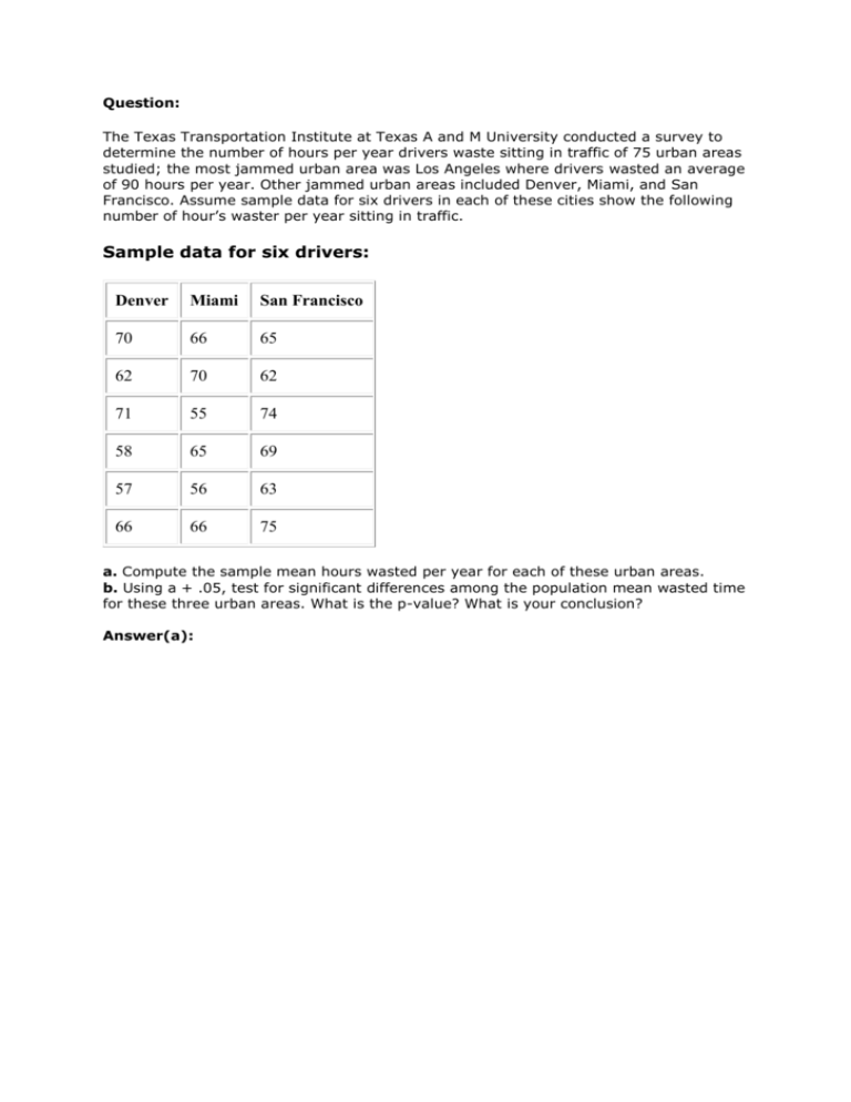
Question:
The Texas Transportation Institute at Texas A and M University conducted a survey to
determine the number of hours per year drivers waste sitting in traffic of 75 urban areas
studied; the most jammed urban area was Los Angeles where drivers wasted an average
of 90 hours per year. Other jammed urban areas included Denver, Miami, and San
Francisco. Assume sample data for six drivers in each of these cities show the following
number of hour’s waster per year sitting in traffic.
Sample data for six drivers:
Denver
Miami
San Francisco
70
66
65
62
70
62
71
55
74
58
65
69
57
56
63
66
66
75
a. Compute the sample mean hours wasted per year for each of these urban areas.
b. Using a + .05, test for significant differences among the population mean wasted time
for these three urban areas. What is the p-value? What is your conclusion?
Answer(a):
Mean of Denver =
=
=
= 64
Similarly the other for the other cities can be calculated. Hence we have
Ø Mean of Denver = 64 hours
Ø Mean of Miami = 63 hours
Ø Mean of San Francisco = 68 hours
Answer(b):
In order to test whether there is difference in the mean hours wasted by the car drivers,
we have to perform as ANOVA (Analysis of Variance).
Null hypothesis:
H0:
That is there is no significance difference among the mean hours wasted by the drivers
in the three cities.
Alternate hypothesis:
H1: Not all population means are equal.
That is there is significance difference among the mean hours wasted by the drivers in
the three cities.
The Analysis of Variance is carried out using Microsoft Excel. The steps to be followed
in Microsoft Excel are as follows:
·
Select ‘Data’ from the main menu. Then click ‘Data Analysis’.
·
Select ‘ANOVA – one factor’ from the analysis tools.
·
Input the given data range in ‘input range’.
·
Then click ‘OK’ to get the result.
The above mentioned steps are followed using Microsoft Excel and the output is given
below:
Anova: Single
Factor
SUMMARY
Groups
Denvver
Miami
San Francisco
ANOVA
Source of Variation
Between Groups
Within Groups
Total
Count
6
6
6
SS
Sum
384
378
408
df
Average
MS
Variance
64
35.6
63
36.8
68
31.2
84
518
F
P-value F crit
2
42 1.216216 0.323966 3.68232
15 34.53333333
602
17
Hence the P-value corresponding to F test statistic is 0.323966.
Statistical decision:
From the Anova table, we see that that P-value (0.323966) corresponding to the F test
statistic is greater than 0.05 (level of significance). Hence we do not reject the null
hypothesis at 0.05 level of significance.
i.e:, there is no significance difference among the mean hours wasted by the
drivers in the three cities.